Page 229 - Numerical Analysis Using MATLAB and Excel

Chapter 6 Fourier, Taylor, and Maclaurin Series

3rd harmonic
2nd harmonic
Fundamental

c
1
a
0.5
b b
0
−a
-0.5
−c
-1
T/2
0 2 4 T/2 6 8 T/2 10 12
(for fundamental) (for 2nd harmonic) (for 3rd harmonic)
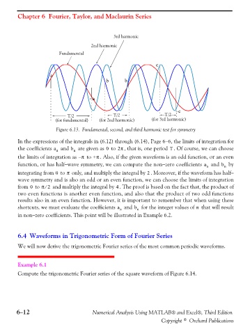
Figure 6.13. Fundamental, second, and third harmonic test for symmetry

In the expressions of the integrals in (6.12) through (6.14), Page 6−6, the limits of integration for
T
0
the coefficients a n and b n are given as to 2π , that is, one period . Of course, we can choose
the limits of integration as π– to +π . Also, if the given waveform is an odd function, or an even
function, or has half−wave symmetry, we can compute the non−zero coefficients a n and b n by
π
integrating from to only, and multiply the integral by . Moreover, if the waveform has half−
2
0
wave symmetry and is also an odd or an even function, we can choose the limits of integration
from to π 2⁄ and multiply the integral by . The proof is based on the fact that, the product of
4
0
two even functions is another even function, and also that the product of two odd functions
results also in an even function. However, it is important to remember that when using these
n
shortcuts, we must evaluate the coefficients a n and b n for the integer values of that will result
in non−zero coefficients. This point will be illustrated in Example 6.2.

6.4 Waveforms in Trigonometric Form of Fourier Series

We will now derive the trigonometric Fourier series of the most common periodic waveforms.

Example 6.1
Compute the trigonometric Fourier series of the square waveform of Figure 6.14.

6−12 Numerical Analysis Using MATLAB® and Excel®, Third Edition
Copyright © Orchard Publications