Page 75 - Numerical Analysis Using MATLAB and Excel

Chapter 2 Root Approximations

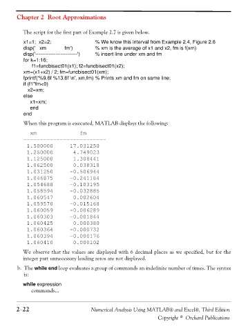
The script for the first part of Example 2.7 is given below.

x1=1; x2=2; % We know this interval from Example 2.4, Figure 2.6
disp(' xm fm') % xm is the average of x1 and x2, fm is f(xm)
disp('-------------------------') % insert line under xm and fm
for k=1:16;
f1=funcbisect01(x1); f2=funcbisect01(x2);
xm=(x1+x2) / 2; fm=funcbisect01(xm);
fprintf('%9.6f %13.6f \n', xm,fm) % Prints xm and fm on same line;
if (f1*fm<0)
x2=xm;
else
x1=xm;
end
end
When this program is executed, MATLAB displays the following:

xm fm
-------------------------
1.500000 17.031250
1.250000 4.749023
1.125000 1.308441
1.062500 0.038318
1.031250 -0.506944
1.046875 -0.241184
1.054688 -0.103195
1.058594 -0.032885
1.060547 0.002604
1.059570 -0.015168
1.060059 -0.006289
1.060303 -0.001844
1.060425 0.000380
1.060364 -0.000732
1.060394 -0.000176
1.060410 0.000102
We observe that the values are displayed with 6 decimal places as we specified, but for the
integer part unnecessary leading zeros are not displayed.
b. The while end loop evaluates a group of commands an indefinite number of times. The syntax
is:

while expression
commands...

2−22 Numerical Analysis Using MATLAB® and Excel®, Third Edition
Copyright © Orchard Publications