Page 73 - Numerical Analysis Using MATLAB and Excel

Chapter 2 Root Approximations

The objective is to find two values of x, say x 1 and x 2 , so that fx ) ( 1 and fx ) ( 2 have opposite
signs, that is, either fx ( 1 ) > 0 and fx ) ( 2 < 0 , or fx ) ( 1 < 0 and fx ) ( 2 > 0 . If any of these two condi-
tions is satisfied, we can compute the midpoint x of the interval x ≤ 1 x ≤ x 2 with
m
x + x
1
x m = ----------------- 2 (2.18)
2
Knowing x m , we can find fx ) ( m . Then, the following decisions are made:

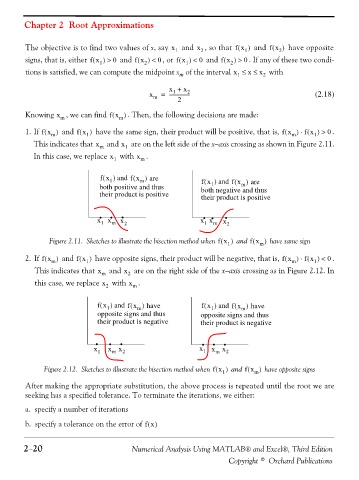
1. If fx ( m ) and fx ) ( 1 have the same sign, their product will be positive, that is, fx ) ( m fx ) ( ⋅ 1 > . 0

This indicates that x m and x 1 are on the left side of the x−axis crossing as shown in Figure 2.11.
In this case, we replace x 1 with x m .

fx ( 1 ) an fx (d m ) are fx ( ) and fx ( ) are
1
m
both positive and thus both negative and thus
their product is positive their product is positive

•
• •
x x • m x • 2 x x m x • 2
1
1
Figure 2.11. Sketches to illustrate the bisection method when fx ) ( 1 and fx ) ( m have same sign

2. If fx ( m ) and fx ) ( 1 have opposite signs, their product will be negative, that is, fx ) ( m fx ) ( ⋅ 1 < . 0
This indicates that x m and x 2 are on the right side of the x−axis crossing as in Figure 2.12. In

this case, we replace x 2 with x m .

fx ( 1 ) and fx ( m ) have fx ( 1 ) and fx ( m ) have
opposite signs and thus opposite signs and thus
their product is negative their product is negative

• • • • • •
x 1 x x 2 x 1 x x 2
m
m
Figure 2.12. Sketches to illustrate the bisection method when fx ) ( 1 and fx ) ( m have opposite signs

After making the appropriate substitution, the above process is repeated until the root we are
seeking has a specified tolerance. To terminate the iterations, we either:
a. specify a number of iterations

b. specify a tolerance on the error of fx()

2−20 Numerical Analysis Using MATLAB® and Excel®, Third Edition
Copyright © Orchard Publications