Page 68 - Numerical Analysis Using MATLAB and Excel

Approximations with Spreadsheets

roots_p =
-1.1415 + 0.8212i
-1.1415 - 0.8212i
0.6113 + 0.9476i
0.6113 - 0.9476i
1.0604

Example 2.5
Compute the real roots of the trigonometric function

y = f x() = cos 2x + sin 2x + x 1 (2.16)
–
using Excel.
Solution:

We invoke (open) the spreadsheet of one of the last two examples, that is, poly01.xls or poly02.xls,
and save it with another name, such as poly03.xls.

Since we do not know where real roots (if any) are in the x−axis interval, we arbitrarily choose the
interval 1 ≤– x ≤ 6 . Then, we enter −1.00 and −0.90 in A2 and A3 respectively, Using the Auto-
Fill feature, we fill−in the range A4:A72 and thus we have the interval from −1 to 6 in increments
of 0.10. Next, we select B2 and we enter the formula for the given equation, i.e.,

=COS(2*A2)+SIN(2*A2)+A2−1

and we copy this formula to B3:B62.

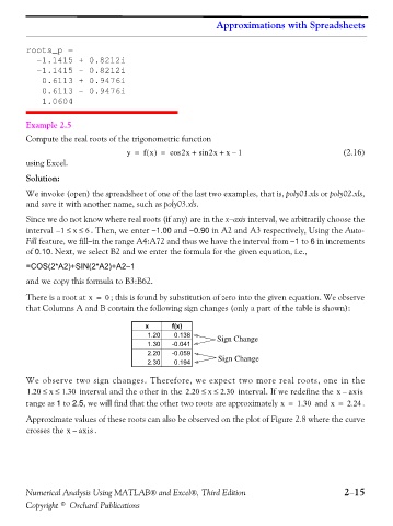
There is a root at x = 0 ; this is found by substitution of zero into the given equation. We observe
that Columns A and B contain the following sign changes (only a part of the table is shown):

x f(x)
1.20 0.138 Sign Change
1.30 -0.041
2.20 -0.059
2.30 0.194 Sign Change

We observe two sign changes. Therefore, we expect two more real roots, one in the
1.20 ≤≤ 1.30 interval and the other in the 2.20 ≤≤ 2.30 interval. If we redefine the x – axis
x
x
range as 1 to 2.5, we will find that the other two roots are approximately x = 1.30 and x = 2.24 .
Approximate values of these roots can also be observed on the plot of Figure 2.8 where the curve
crosses the x – axis .

Numerical Analysis Using MATLAB® and Excel®, Third Edition 2−15
Copyright © Orchard Publications