Page 67 - Numerical Analysis Using MATLAB and Excel

Chapter 2 Root Approximations

3. From the Chart menu we select Value (Y) axis, and we click on the small box next to it. Then,
on the Format axis menu, we click on the Scale tab and make the following entries:

Minimum: −1.0
Maximum: 1.0
Major unit: 0.5
Minor unit: 0.1
4. We click on the Titles tab and make the following entries:

Chart title: f(x) = the given equation (or whatever we wish)
Value (X) axis: x (or whatever we wish)
Value (Y) axis: y=f(x) (or whatever we wish)
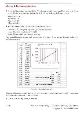
Our spreadsheet now should look like the one in Figure 2.7 and we see that one real root is
approximately 1.06.

x f(x)
3
f(x) = 3x - 2x + 6x - 8
5
1.00 -1.000
1.05 -0.186
1.00
1.10 0.770
1.15 1.892 0.50
1.20 3.209
1.25 4.749 f(x) 0.00
1.30 6.545 -0.50
1.35 8.631
1.40 11.047 -1.00
1.45 13.832 1.00 1.02 1.04 1.06 1.08 1.10
1.50 17.031 x
1.55 20.692
1.60 24.865
1.65 29.605
1.70 34.970 x f(x)
1.75 41.021 1.00 -1.000
1.80 47.823 Real Root between 1.05 -0.186
1.85 55.447 1.10 0.770
1.90 63.965 1.15 1.892
1.95 73.455 1.20 3.209
2.00 84.000 f(x) = − 0.007 at x = 1.06

Figure 2.7. Graph for Example 2.4

Since no other roots are indicated on the plot, we suspect that the others are complex conjugates.
We confirm this with MATLAB as follows:

p = [ 3 0 −2 0 6 −8]; roots_p=roots(p)

2−14 Numerical Analysis Using MATLAB® and Excel®, Third Edition
Copyright © Orchard Publications