Page 71 - Numerical Analysis Using MATLAB and Excel

Chapter 2 Root Approximations

A B C D E F G H
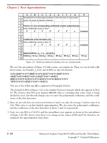
1 Spreadsheet for finding approximations of the real roots of polynomials
2 up the 7th power by Newton's Method.
3
4 Powers of x and corresponding coefficients of given polynomial p(x)
5 Enter coefficients of p(x) in Row 7
6 x 7 x 6 x 5 x 4 x 3 x 2 x Constant
7
8
9 Coefficients of the derivative p'(x)
10 Enter coefficients of p'(x) in Row 12
11 x 6 x 5 x 4 x 3 x 2 x Constant
12
13
14 Approximations: x n+1 = x n − p(x n )/p'(x n )
15 Initial (x 0 ) 1st (x 1 ) 2nd (x 2 ) 3rd (x 3 ) 4th (x 4 ) 5th (x 5 ) 6th (x 6 ) 7th (x 7 )
16

Figure 2.9. Model spreadsheet for finding real roots of polynomials.

We save the spreadsheet of Figure 2.9 with a name, say template.xls. Then, we save it with a dif-
ferent name, say Example_2_6.xls, and in B16 we type the formula
=A16-($A$7*A16^7+$B$7*A16^6+$C$7*A16^5+$D$7*A16^4
+$E$7*A16^3+$F$7*A16^2+$G$7*A16^1+$H$7)/
($B$12*A16^6+$C$12*A16^5+$D$12*A16^4+$E$12*A16^3
+$F$12*A16^2+$G$12*A16^1+$H$12)

The use of the dollar sign ($) is explained in Paragraph 4 below.
The formula in B16 of Figure 2.10, is the familiar Newton’s formula which also appears in Row
14. We observe that B16 now displays #DIV/0! (this is a warning that some value is being
divided by zero), but this will change once we enter the polynomial coefficients, and the coeffi-
cients of the first derivative.

2. Since we are told that one real root is between 4 and 6, we take the average 5 and we enter it in
A16. This value is our first (initial) approximation. We also enter the polynomial coefficients,
and the coefficients of the first derivative in Rows 7 and 12 respectively.
3. Next, we copy B16 to C16:F16 and the spreadsheet now appears as shown in the spreadsheet
of Figure 2.10. We observe that there is no change in the values of E16 and F16; therefore, we
terminate the approximation steps there.

2−18 Numerical Analysis Using MATLAB® and Excel®, Third Edition
Copyright © Orchard Publications