Page 65 - Numerical Analysis Using MATLAB and Excel

Chapter 2 Root Approximations

x f(x)
3
2
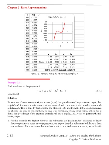
0.00 -12.000 f(x) = x - 7x + 16x - 12
0.05 -11.217
0.10 -10.469 1.00
0.15 -9.754 0.75
0.20 -9.072 0.50
0.25
0.25 -8.422 f(x) 0.00
0.30 -7.803 -0.25
0.35 -7.215 -0.50
0.40 -6.656 -0.75
0.45 -6.126 -1.00
0.50 -5.625 0 1 2 3 4 5
0.55 -5.151 x
0.60 -4.704
0.65 -4.283
0.70 -3.887 x f(x) x f(x)
0.75 -3.516 1.90 -0.011 2.90 -0.081
0.80 -3.168 1.95 -0.003 2.95 -0.045
0.85 -2.843 Roots 2.00 0.000 3.00 0.000
0.90 -2.541 2.05 -0.002 3.05 0.055
0.95 -2.260 2.10 -0.009 3.10 0.121
1.00 -2.000 f(x) =0 at x=2 (double root) and at x=3
Figure 2.5. Modified plot of the equation of Example 2.3.

Example 2.4
Find a real root of the polynomial

3
5
y = f x() = 3x – 2x + 6x – 8 (2.15)
using Excel.
Solution:

To save lots of unnecessary work, we invoke (open) the spreadsheet of the previous example, that
is, poly01.xls (or any other file name that was assigned to it), and save it with another name such
as poly02.xls. This is done by first opening the file poly01.xls, and from the File drop down menu,
we choose the Save as option; then, we save it as poly02.xls, or any other name. When this is
done, the spreadsheet of the previous example still exists as poly01.xls. Next, we perform the fol-
lowing steps:
1. For this example, the highest power of the polynomial is 5 (odd number), and since we know
that complex roots occur in conjugate pairs, we expect that this polynomial will have at least
one real root. Since we do not know where a real root is in the x−axis interval, we arbitrarily

2−12 Numerical Analysis Using MATLAB® and Excel®, Third Edition
Copyright © Orchard Publications