Page 60 - Numerical Analysis Using MATLAB and Excel

Approximations with Spreadsheets

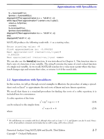
fx = funcnewt01(x);
fprimex = funcnewt02(x);
disp(sprintf('First approximation is x = %9.6f \n', x))
while input('Next approximation? (<enter>=no,1=yes)');
xnext=x−fx/fprimex;
x=xnext;
fx=funcnewt01(x);
fprimex=funcnewt02(x);
disp(sprintf('Next approximation is x = %9.6f \n', x))
end;
disp(sprintf('%9.6f \n', x))
–
MATLAB produces the following result with 1 as a starting value.

Enter starting value: −1
First approximation is: -0.894010
Next approximation? (<enter>=no,1=yes)1
-0.895225
Next approximation? (<enter>=no,1=yes) <enter>
We can also use the fzero(f,x) function. It was introduced in Chapter 1. This function tries to
find a zero of a function of one variable. The string f contains the name of a real−valued function
of a single real variable. As we recall, MATLAB searches for a value near a point where the func-
tion f changes sign and returns that value, or returns NaN if the search fails.

2.2 Approximations with Spreadsheets

In this section, we will go through several examples to illustrate the procedure of using a spread-
*
sheet such as Excel to approximate the real roots of linear and non−linear equations.
We recall that there is a standard procedure for finding the roots of a cubic equation; it is
included here for convenience.

A cubic equation of the form
3
2
y + py + qy + r = 0 (2.8)
can be reduced to the simpler form
3
x + ax + b = 0 (2.9)
where

* We will illustrate our examples with Excel, although others such as Lotus 1−2−3, and Quattro can also be used. Hence-
forth, all spreadsheet commands and formulas that we will be using, will be those of Excel.

Numerical Analysis Using MATLAB® and Excel®, Third Edition 2−7
Copyright © Orchard Publications