Page 56 - Numerical Analysis Using MATLAB and Excel

Newton’s Method for Root Approximation

We chose this interval because the given equation asks for the square root of ; we expect this
5
value to be a value between and . For other functions, where the interval may not be so obvi-
3
2
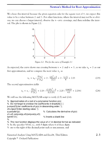
ous, we can choose a larger interval, observe the x – axis crossings, and then redefine the inter-
val. The plot is shown in Figure 2.2.

15

10

5

0

-5
-4 -2 0 2 4
Figure 2.2. Plot for the curve of Example 2.1

As expected, the curve shows one crossing between x = 2 and x = 3 , so we take x = 2 as our
0
first approximation, and we compute the next value x 1 as

fx ) ( 2 () – 5 – ( 1 )
2
0
x = x – --------------- = 2 – ------------------- = 2 – ----------- = 2.25 (2.5)
1
0
22()
)
f ' x (
4
0
The second approximation yields
fx ) ( ( 2.25 ) 2 – 5 0.0625
1
x = x – --------------- = 2.25 – -------------------------- = 2.25 – ---------------- = 2.2361 (2.6)
1
2
)
)
(
f ' x (
22.25
4.5
1
We will use the following MATLAB script to verify (2.5) and (2.6).
% Approximation of a root of a polynomial function p(x)
% Do not forget to enclose the coefficients in brackets [ ]
p=input('Enter coefficients of p(x) in descending order: ');
x0=input('Enter starting value: ');
q=polyder(p); % Calculates the derivative of p(x)
x1=x0−polyval(p,x0)/polyval(q,x0);
fprintf('\n'); % Inserts a blank line
%
% The next function displays the value of x1 in decimal format as indicated
% by the specifier %9.6f, i.e., with 9 digits where 6 of these digits
% are to the right of the decimal point such as xxx.xxxxxx, and
Numerical Analysis Using MATLAB® and Excel®, Third Edition 2−3
Copyright © Orchard Publications