Page 54 - Numerical Analysis Using MATLAB and Excel

Chapter 2

Root Approximations

T his chapter is an introduction to Newton’s and bisection methods for approximating roots

of linear and non−linear equations. Several examples are presented to illustrate practical
solutions using MATLAB and Excel spreadsheets.

2.1 Newton’s Method for Root Approximation

Newton’s (or Newton−Raphson) method can be used to approximate the roots of any linear or
non−linear equation of any degree. This is an iterative (repetitive procedure) method and it is
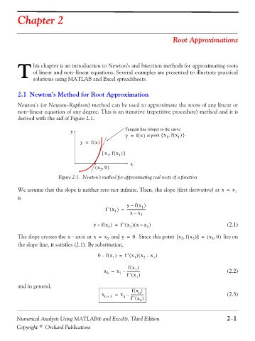
derived with the aid of Figure 2.1.

y Tangent line (slope) to the curve
y = f() at point x fx(,{ x 1 1 ) }
y = f x()

• x fx( ,{ ) }
1 1
• x
( x 0, ) 2
Figure 2.1. Newton’s method for approximating real roots of a function

We assume that the slope is neither zero nor infinite. Then, the slope (first derivative) at x = x 1
is
y f x (– )
1
f ' x ( 1 ) = ---------------------
–
xx
1
y f x (– 1 ) f ' x ) ( = 1 ( xx ) – 1 (2.1)
,
The slope crosses the x – axis at x = x 2 and y = 0 . Since this point x fx(,[ 2 2 ) ] ( = x 0 ) lies on
2
the slope line, it satisfies (2.1). By substitution,
0 f x (– 1 ) f ' x ) ( = 1 ( x – x ) 1
2
fx ) (
1
x = x – --------------- ) (2.2)
2
1
f ' x (
1
and in general,
fx ) (
n
x n + 1 = x – --------------- ) (2.3)
n
f ' x (
n
Numerical Analysis Using MATLAB® and Excel®, Third Edition 2−1
Copyright © Orchard Publications