Page 58 - Numerical Analysis Using MATLAB and Excel

Newton’s Method for Root Approximation

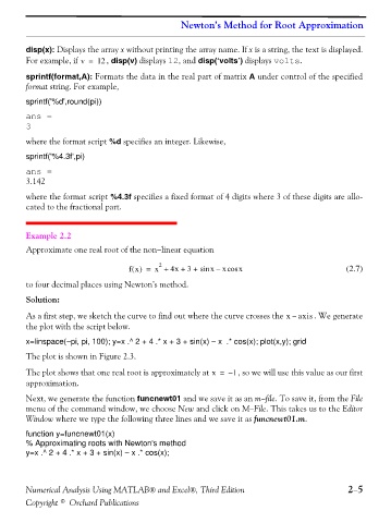
disp(x): Displays the array x without printing the array name. If x is a string, the text is displayed.
For example, if v = 12 , disp(v) displays 12, and disp(‘volts’) displays volts.

sprintf(format,A): Formats the data in the real part of matrix A under control of the specified
format string. For example,

sprintf('%d',round(pi))

ans =
3
where the format script %d specifies an integer. Likewise,

sprintf('%4.3f',pi)
ans =
3.142
where the format script %4.3f specifies a fixed format of 4 digits where 3 of these digits are allo-
cated to the fractional part.

Example 2.2
Approximate one real root of the non−linear equation

2
fx() = x + 4x + + sin x – xcos x (2.7)
3
to four decimal places using Newton’s method.
Solution:

As a first step, we sketch the curve to find out where the curve crosses the x – axis . We generate
the plot with the script below.

x=linspace(−pi, pi, 100); y=x .^ 2 + 4 .* x + 3 + sin(x) − x .* cos(x); plot(x,y); grid
The plot is shown in Figure 2.3.

The plot shows that one real root is approximately at x = – 1 , so we will use this value as our first
approximation.
Next, we generate the function funcnewt01 and we save it as an m−file. To save it, from the File
menu of the command window, we choose New and click on M−File. This takes us to the Editor
Window where we type the following three lines and we save it as funcnewt01.m.

function y=funcnewt01(x)
% Approximating roots with Newton's method
y=x .^ 2 + 4 .* x + 3 + sin(x) − x .* cos(x);

Numerical Analysis Using MATLAB® and Excel®, Third Edition 2−5
Copyright © Orchard Publications