Page 50 - Numerical Analysis Using MATLAB and Excel

Exercises

1.12 Exercises

1. Use MATLAB to compute the roots of the following polynomials:

3
2
a. px() = x + 8x + 10x + 4
5
3
2
4
b. py() = y + 7y + 19y + 25y + 16y + 4
2. Use MATLAB to derive the polynomials having the following roots:
a. 6.5708 – 0.7146 + j0.3132 – 0.7146 j0.3132
–
–
b. Two roots at x = – 2.000 and three roots at x = – 3.000

3. Use MATLAB to evaluate the polynomials below at the specified values.

3
2
a. px() = x + 8x + 10x + 4 at x = 1.25
3
2
4
5
b. py() = y + 7y + 19y + 25y + 16y + 4 at y = – 3.75
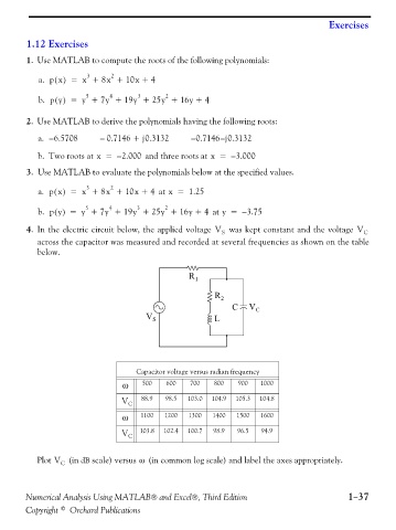
4. In the electric circuit below, the applied voltage V S was kept constant and the voltage V C
across the capacitor was measured and recorded at several frequencies as shown on the table
below.

R 1

R 2
C V C
V S L

Capacitor voltage versus radian frequency
ω 500 600 700 800 900 1000

V C 88.9 98.5 103.0 104.9 105.3 104.8
ω 1100 1200 1300 1400 1500 1600

V C 103.8 102.4 100.7 98.9 96.5 94.9

Plot V C (in dB scale) versus (in common log scale) and label the axes appropriately.ω

Numerical Analysis Using MATLAB® and Excel®, Third Edition 1−37
Copyright © Orchard Publications