Page 82 - Numerical Analysis Using MATLAB and Excel

Solutions to End-of-Chapter Exercises

2.6 Solutions to End-of-Chapter Exercises

1.
a.

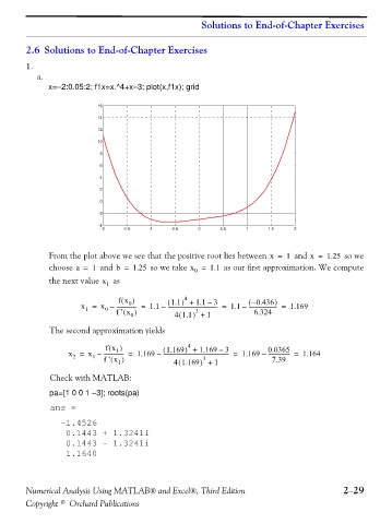
x=−2:0.05:2; f1x=x.^4+x−3; plot(x,f1x); grid

16
14
12
10
8
6
4
2
0
-2

-4
-2 -1.5 -1 -0.5 0 0.5 1 1.5 2

From the plot above we see that the positive root lies between x = 1 and x = 1.25 so we
choose a = 1 and b = 1.25 so we take x = 1.1 as our first approximation. We compute
0
the next value x 1 as

fx ) ( ( 1.1 ) 4 + 1.1 3 – ( 0.436 )
–
0
x = x – --------------- = 1.1 – ------------------------------------- = 1.1 – --------------------- = 1.169
0
1
)
f ' x (
6.324
3
)
(
1
41.1
+
0
The second approximation yields
fx ) ( ( 1.169 ) 4 + 1.169 – 3 0.0365
1
x = x – --------------- = 1.169 – ------------------------------------------------- = 1.169 – ---------------- = 1.164
1
2
f ' x (
)
7.39
3
)
(
+
41.169
1
1
Check with MATLAB:
pa=[1 0 0 1 −3]; roots(pa)
ans =
-1.4526
0.1443 + 1.3241i
0.1443 - 1.3241i
1.1640
Numerical Analysis Using MATLAB® and Excel®, Third Edition 2−29
Copyright © Orchard Publications