Page 86 - Numerical Analysis Using MATLAB and Excel

Solutions to End-of-Chapter Exercises

3.
From Example 2.5,
y = f x() = cos 2x + sin 2x + x 1
–
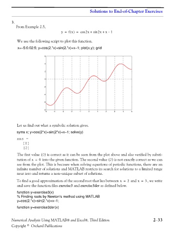
We use the following script to plot this function.

x=−5:0.02:5; y=cos(2.*x)+sin(2.*x)+x−1; plot(x,y); grid

6

4

2

0

-2

-4

-6

-8
-5 -4 -3 -2 -1 0 1 2 3 4 5

Let us find out what a symbolic solution gives.

syms x; y=cos(2*x)+sin(2*x)+x−1; solve(y)
ans =
[0]
[2]
The first value (0) is correct as it can be seen from the plot above and also verified by substi-
tution of x = 0 into the given function. The second value (2) is not exactly correct as we can
see from the plot. This is because when solving equations of periodic functions, there are an
infinite number of solutions and MATLAB restricts its search for solutions to a limited range
near zero and returns a non−unique subset of solutions.

To find a good approximation of the second root that lies between x = 2 and x = 3 , we write
and save the function files exercise3 and exercise3der as defined below.

function y=exercise3(x)
% Finding roots by Newton's method using MATLAB
y=cos(2.*x)+sin(2.*x)+x−1;
function y=exercise3der(x)

Numerical Analysis Using MATLAB® and Excel®, Third Edition 2−33
Copyright © Orchard Publications