Page 83 - Numerical Analysis Using MATLAB and Excel

Chapter 2 Root Approximations

b.

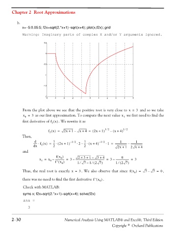
x=−5:0.05:5; f2x=sqrt(2.*x+1)−sqrt(x+4); plot(x,f2x); grid
Warning: Imaginary parts of complex X and/or Y arguments ignored.

0.5

0

-0.5

-1

-1.5

-2
-5 -4 -3 -2 -1 0 1 2 3 4 5

From the plot above we see that the positive root is very close to x = 3 and so we take
x = 3 as our first approximation. To compute the next value x 1 we first need to find the
0
first derivative of f x() . We rewrite it as
2
⁄
⁄
f x() = 2x + 1 – x + 4 = ( 2x + 1 ) 12 – ( x + 4 ) 12
2
Then,
d
1
1
⁄
⁄
------ f x()⋅ 1 - ⋅ 2x + 1 ) – 1 2 2 ⋅ 1 - ⋅ x + 4 ) – 1 2 ⋅ 1 = ------------------- – -------------------
-- ( =
-- ( –
dx 2 2 2 2x + 1 2x + 4
and
fx ) ( 2 × 3 + – 3 + 4 0
1
0
x = x – --------------- = 3 – ------------------------------------------------ = 3 – ---------------------- = 3
1
0
)
f ' x (
) ⁄
1 ⁄
) ⁄
1 (
2 7
7 1 (–
2 7
0
Thus, the real root is exactly x = 3 . We also observe that since fx ) ( 0 = 7 – 7 = , 0
there was no need to find the first derivative f ' x( 0 . )
Check with MATLAB:
syms x; f2x=sqrt(2.*x+1)−sqrt(x+4); solve(f2x)
ans =
3
2−30 Numerical Analysis Using MATLAB® and Excel®, Third Edition
Copyright © Orchard Publications