Page 223 - Numerical Analysis and Modelling in Geomechanics

204 I.-M.LEE AND D.-H.KIM
Formulation of extended Bayesian method
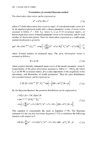
The observation data vector can be expressed as:

(7.8)

k
*u
where u =field observation data vector at step k, u =calculated results vector at k
k
by an employed physical model with a chosen parameter vector, ε =error vector
assumed to follow ε k ~ N(0, V ), where V u is an N×N covariance matrix, x=
u
known input data vector, θ=model parameter vector to be estimated, and N= total
number of observation points. Then the observation expressed as a multivariate
normal distribution is given by
(7.
9)

where K=total number of measured steps. The prior information vector is
assumed as follows:
(7.10)

where p=prior (initially estimated) mean vector of the model parameter vector θ,
δ=uncertainty of the prior information assumed to follow δ ~ N(0,V /β) where
p
V is an M×M covariance matrix, β=a scalar adjustment of the magnitude of the
p
uncertainty, and M=number of model parameters. Then the prior distribution,
also assumed normal, can be expressed as:

(7.11)

By the Bayesian theorem, the posterior distribution can be expressed as:

(7.12)

This equation is conceptually the same as Equation (7.7b). The Bayesian
estimator θ is the one that maximizes Equation (7.12) or minimizes the following
function with respect to θ:

(7.13)