Page 13 - Numerical Methods for Chemical Engineering

2 1 Linear algebra

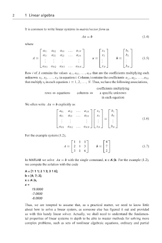
It is common to write linear systems in matrix/vector form as

Ax = b (1.4)
where

     
a 11 a 12 a 13 ... a 1N x 1 b 1
...
a 21 a 22 a 23 a 2N x 2 b 2
     


A =  . . .  x =  .  b =  .  (1.5)

 . . . . . . .   . .   . . 
.


. 
a N1 a N2 a N3 ... a NN x N b N
Row i of A contains the values a i1 , a i2 ,..., a iN that are the coefficients multiplying each
unknown x 1 , x 2 ,..., x N in equation i. Column j contains the coefficients a 1 j , a 2 j ,..., a Nj
that multiply x j in each equation i = 1, 2,..., N. Thus, we have the following associations,
coefficients multiplying
rows ⇔ equations columns ⇔ a specific unknown
in each equation
We often write Ax = b explicitly as
     
a 11 a 12 ... a 1N x 1 b 1
a 21 a 22 a 2N x 2 b 2
 ...     
 . .      (1.6)

 . . . . .   .  =  . 
.
.
.
 . 
.   . 
a N1 a N2 ... a NN x N b N
For the example system (1.2),
   
111 4
7
A =  213  b =   (1.7)
316 2
In MATLAB we solve Ax = b with the single command, x=A\b. For the example (1.2),
we compute the solution with the code
A=[111;213;316];
b = [4; 7; 2];
x=A\b,
x=
19.0000
-7.0000
-8.0000
Thus, we are tempted to assume that, as a practical matter, we need to know little
about how to solve a linear system, as someone else has figured it out and provided
us with this handy linear solver. Actually, we shall need to understand the fundamen-
tal properties of linear systems in depth to be able to master methods for solving more
complex problems, such as sets of nonlinear algebraic equations, ordinary and partial