Page 15 - Numerical Methods for Chemical Engineering

4 1 Linear algebra

e 2 1

v 2
v
v 1
0
e 1 1
v
e 1
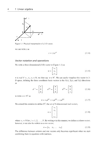
Figure 1.1 Physical interpretation of a 3-D vector.

we can write z as
z =|z|e iθ (1.14)

Vector notation and operations
We write a three-dimensional (3-D) vector v (Figure 1.1) as
 
v 1
v =  v 2  (1.15)
v 3
3
v is real if v 1 ,v 2 ,v 3 ∈ ; we then say v ∈ . We can easily visualize this vector in 3-
D space, defining the three coordinate basis vectors in the 1(x), 2(y), and 3(z) directions
as
     
1 0 0
0
1
0
e [1] =   e [2] =   e [3] =   (1.16)
0 0 1
3
to write v ∈ as
v = v 1 e [1] + v 2 e [2] + v 3 e [3] (1.17)
N
We extend this notation to define , the set of N-dimensional real vectors,
 
v 1
v 2
 
(1.18)
 
v =  . 
.
 . 
v N
where v j ∈ for j = 1, 2,..., N. By writing v in this manner, we define a column vector;
however, v can also be written as a row vector,
v 2 ... v N ] (1.19)
v = [v 1
The difference between column and row vectors only becomes significant when we start
combining them in equations with matrices.