Page 193 - Numerical Methods for Chemical Engineering

182 4 Initial value problems

2
A
1
B
1
1
ct
12
atin 1
cncentr

2

2 1
tie t
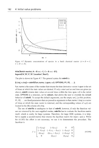
Figure 4.7 Dynamic concentrations of species in a batch chemical reactor (A + B → C,
C + B → D).

title(‘Batch reactor,A+B==> C,C+B==> D’);
legend(‘A’,‘B’,‘C’,‘D’,‘Location’,‘Best’);

The plot is shown in Figure 4.7. The general syntax for ode45 is
[t traj, x traj] = ode45(fun name, t span, x 0, OPTIONS, P1, P2, . . .);

fun name is the name of the routine that returns the time derivative vector. t span is the set
of times at which the state values are desired. If only a start and an end time are given (as
above), ode45 returns state values at several times within the time span. x 0 is the initial
state. OPTIONS is a structure, set by odeset, that allows the user to override the default
behavior of ode45. To accept the default arguments, use the empty set[]at this position.
P1, P2,...arefixed parameters that are passed as arguments to fun name. t traj is a vector
of times at which the state vector is returned, and the corresponding values of x k (t) are
located in the kth column of x traj.
The use of ode15s is analogous to that of ode45; however, if only the function val-
ues are returned by the user-supplied routine, ode15s has to evaluate the Jacobian matrix
itself, which is costly for large systems. Therefore, for large ODE systems, it is help-
ful to supply a second routine that returns the Jacobian matrix for input t and x. While
for (4.143) the effort is not necessary, we use it to demonstrate the procedure. The
Jacobian is

(−k 1 c B ) (−k 1 c A ) 0 0
 
(−k 1 c B )(−k 1 c A − k 2 c C )(−k 2 c B )0
 
J =   (4.144)
(k 1 c B ) (k 1 c A − k 2 c C ) (−k 2 c B )0
 
0 (k 2 c C ) (k 2 c B ) 0