Page 197 - Numerical Methods for Chemical Engineering

186 4 Initial value problems

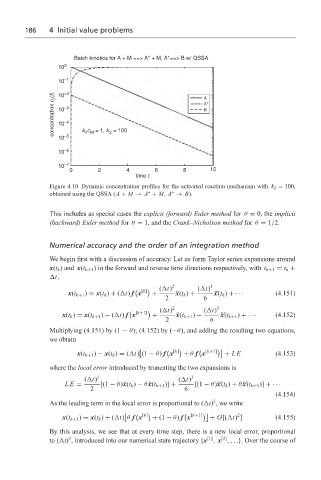
Figure 4.10 Dynamic concentration profiles for the activated reaction mechanism with k 2 = 100,
∗
∗
obtained using the QSSA (A + M → A + M, A → B).
This includes as special cases the explicit (forward) Euler method for θ = 0, the implicit
(backward) Euler method for θ = 1, and the Crank–Nicholson method for θ = 1/2.

Numerical accuracy and the order of an integration method

We begin first with a discussion of accuracy. Let us form Taylor series expansions around
x(t k ) and x(t k+1 ) in the forward and reverse time directions respectively, with t k+1 = t k +
t,
( t) 2 ( t) 3
[k]
x(t k+1 ) = x(t k ) + ( t) f x + ¨ x(t k ) + ¨ x˙(t k ) +· · · (4.151)
2 6
( t) 2 ( t) 3
[k+1]
x(t k ) = x(t k+1 ) − ( t) f x + ¨ x(t k+1 ) − ¨ x˙(t k+1 ) +· · · (4.152)
2 6
Multiplying (4.151) by (1 − θ), (4.152) by (−θ), and adding the resulting two equations,
we obtain

[k] [k+1]
x(t k+1 ) − x(t k ) = ( t) (1 − θ) f x + θ f x + LE (4.153)
where the local error introduced by truncating the two expansions is
( t) 2 ( t) 3
LE = [(1 − θ)¨x(t k ) − θ ¨x(t k+1 )] + [(1 − θ)¨x˙(t k ) + θ ¨x˙(t k+1 )] +· · ·
2 6
(4.154)
2
As the leading term in the local error is proportional to ( t) , we write
[k] [k+1] 2
x(t k+1 ) = x(t k ) + ( t) θ f x + (1 − θ) f x + O[( t) ] (4.155)
By this analysis, we see that at every time step, there is a new local error, proportional
[2]
2
[1]
to ( t) , introduced into our numerical state trajectory {x , x ,...}. Over the course of