Page 195 - Numerical Methods for Chemical Engineering

184 4 Initial value problems

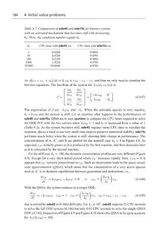
Table 4.2 Comparison of ode45 and ode15s for kinetics system
with an activated mechanism that becomes stiff with increasing
k 2 . Here, the condition number equals k 2

k 2 CPU time with ode45 (s) CPU time with ode15s (s)
1 0.0200 0.0401
10 0.0200 0.0901
100 0.2103 0.0801
1000 1.8226 0.0701
10 000 24.8648 0.0701

As d[c A + c A + c B ]/dt = 0, c B = c A0 − c A − c A and thus we only need to simulate the
∗
∗
first two equations. The Jacobian of the system for {c A (t), c A (t)} is
∗
 
∂ f 1 ∂ f 1

 ∂c A ∂c A ∗  −k 1 c M 0
J =   = (4.147)
  k 1 c M −k 2
∂ f 2 ∂ f 2
∂c A ∂c A ∗
The eigenvalues of J are −k 1 c M and −k 2 . When the activated species is very reactive,
k 2 k 1 c M and the system is stiff. Let us examine what happens to the performances of
ode45 and ode15s. QSSA ex.m uses cputime to compare the CPU times required to solve
the ODE-IVP with the two solvers when k 1 c M = 1 and k 2 is increased from a value of 1
(Table 4.2). As the system becomes stiff, ode45 requires more CPU time to simulate the
response, due to a need to use very small time steps to preserve numerical stability. ode15s
performs much better when the system is stiff, showing little change in performance. The
*
concentrations of A, A , and B are plotted for the nonstiff case k 2 = 1 in Figure 4.8. As
expected, c A* initially grows as it is produced by the first reaction, and then decreases later
as it is consumed by the second reaction.
For the stiff case k 2 = 100, the dynamic concentration profiles are very different (Figure
4.9). Except for a very short initial period where c A increases rapidly from c A 0 = 0, it
*
∗
appears that c A remains proportional to c A . Such an observation leads to the quasi-steady
*
state approximation (QSSA), which states that the concentration of a very active species
*
such as A is in dynamic equilibrium between generation and destruction; i.e.,

dc A ∗ k 1 c M
= k 1 c M c A − k 2 c A ≈ 0 ⇒ c A ≈ c A (4.148)
∗
∗
dt k 2
With the QSSA, the system reduces to a single ODE,

dc A k 1 c M
∗
=−k 1 c M c A c A0 = 1 c A = c A c B = c A0 − c A − c A ∗ (4.149)
dt k 2
4
that is solved by ode45 with little difficulty. For k 2 = 10 , ode45 requires 25 CPU seconds
to solve the full ODE system (4.146) but only 0.03 CPU seconds to solve the single QSSA
ODE (4.149). Inspection of Figure 4.9 and Figure 4.10 shows the QSSA to be quite accurate
for k 2 /(k 1 c M ) = 100.