Page 208 - Numerical Methods for Chemical Engineering

Differential-algebraic equation (DAE) systems 197

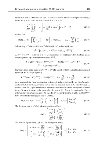
In the sum over k, all terms with k =−1 evaluate to zero, because in the product over p,a
factor for p =−1 contributes a value of 1 + p = 0. As
 
j−2 j−2 j−2 j−1
0 0 0
 
(1 + p) = (1 + p) = l = ( j − 1)! (4.203)

k=−1 p=−1 p=0 l=1
p =k
we find that
m h +1 m h +1
(
1 1
δ ˙π(1) = δπ(1) ( j − 1)! = δπ(1)α −1 α −1 = (4.204)
j! j
j=1 j=1
(c)
(p)
Substituting ˙π (1) = δ ˙π(1) + ˙π (1) into (4.194) and using (4.204),
(p)

M [k+1] α −1 δπ(1) + ˙π (1) = ( t) f x [k+1] (4.205)
(c)
(p)
As x [k+1] = π (1) = δπ(1) + π (1), we substitute for δπ(1) in (4.205) to obtain a non-
linear algebraic equation for the new state x [k+1] ,
[k+1] [k+1] [k+1] [k+1] [k+1] [k]
0 = g x = α −1 M x − ( t) f x − M U
(4.206)
(p)
(p)
U [k] = α −1 π (1) − ˙π (1)
Starting with an initial guess of x [k+1,0] = π (p) (1), we solve (4.206) using Newton’s method,
for which the Jacobian matrix is
∂g ∂ f

B [k+1] = α −1 M x [k+1] − ( t)J x [k+1] B = J = (4.207)
∂x T ∂x T
As x changes little from one iteration to the next and α −1 is fixed by m h (fixed leading-
coefficient BDF method), B varies slowly and we can save much CPU time through LU
factorization. This algorithm marches forward in time similarly to an ODE system; however,
for the Newton iterations to be successful, the matrix B [k+1] must be nonsingular. This is
unfortunately not always the case. We can identify the condition that must be met for B [k+1]
to be invertible for the special case of (4.188),

I 0 y F(y, z)
M(x)˙x = f (x) M = x = f (x) = (4.208)
0 0 z G(y, z)
The Jacobian matrix of f (x) takes the partitioned form
 
∂ F ∂ F
 ∂y T ∂z T 
(4.209)
 

J(x) = 
∂G ∂G

 
∂y T ∂z T
The Newton update matrix (4.207) for this system is then
 
∂ F ∂ F
α −1 I − ( t) −( t)
 ∂y T ∂z T 
B 11 B 12
 
 = (4.210)
B(x) = 
∂G ∂G B 21 B 22

 
−( t) −( t)
∂y T ∂z T