Page 212 - Numerical Methods for Chemical Engineering

Differential-algebraic equation (DAE) systems 201

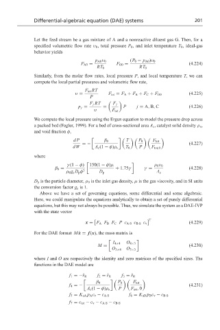
Let the feed stream be a gas mixture of A and a nonreactive diluent gas G. Then, for a
specified volumetric flow rate υ 0 , total pressure P 0 , and inlet temperature T 0 , ideal-gas
behavior yields

p A0 υ 0 (P 0 − p A0 )υ 0
F A0 = F G0 = (4.224)
RT 0 RT 0
Similarly, from the molar flow rates, local pressure P, and local temperature T, we can
compute the local partial pressures and volumetric flow rate,
F tot RT
υ = F tot = F A + F B + F C + F G0 (4.225)
P
F j RT F j
p j = = P j = A, B, C (4.226)
υ F tot
We compute the local pressure using the Ergun equation to model the pressure drop across
a packed bed (Fogler, 1999). For a bed of cross-sectional area A c , catalyst solid density ρ s ,
and void fraction φ,

dP β 0 T P 0 F tot
=− (4.227)
dW A c (1 − φ)ρ s T 0 P F tot,0
where
γ (1 − φ) 150(1 − φ)µ ρ 0 υ 0
β 0 = + 1.75γ γ = (4.228)
ρ 0 g c D p φ 3 D p A c
D p is the particle diameter, ρ 0 is the inlet gas density, µ is the gas viscosity, and in SI units
the conversion factor g c is 1.
Above we have a set of governing equations, some differential and some algebraic.
Here, we could manipulate the equations analytically to obtain a set of purely differential
equations, but this may not always be possible. Thus, we simulate the system as a DAE-IVP
with the state vector
T

x = F A F B F C Pc A·S c B·S c v (4.229)
For the DAE format M ˙x = f (x), the mass matrix is

I 4×4 O 4×3
M = (4.230)
O 3×4 O 3×3
where I and O are respectively the identity and zero matrices of the specified sizes. The
functions in the DAE model are

f 1 =−ˆ r R f 2 = ˆ r R f 3 = ˆ r R

β 0 P 0 F tot
f 4 =− (4.231)
A c (1 − φ)ρ s P F tot , 0
f 5 = K aA p A c v − c A·S f 6 = K aB p B c v − c B·S
f 7 = c tot − c v − c A·S − c B·S