Page 302 - Numerical Methods for Chemical Engineering

Discretized PDEs with more than two spatial dimensions 291

cnate radient iteratins wit
n recnditiner 1
ner c iteratins 1 1 1 1 1 1 2 1 1 1
2

dr terance in cinc

er nd n nn c A
r cinc 1 nn A

1
nn 1 1 1 1 1 2 1 1 1
dr terance in cinc
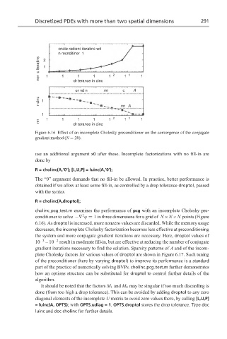
Figure 6.16 Effect of an incomplete Cholesky preconditioner on the convergence of the conjugate
gradient method (N = 20).

use an additional argument x0 after these. Incomplete factorizations with no fill-in are
done by
R = cholinc(A,‘0’); [L,U,P] = luinc(A,‘0’);

The “0” argument demands that no fill-in be allowed. In practice, better performance is
obtained if we allow at least some fill-in, as controlled by a drop tolerance droptol, passed
with the syntax
R = cholinc(A,droptol);

cholinc pcg test.m examines the performance of pcg with an incomplete Cholesky pre-
2
conditioner to solve −∇ ϕ = 1 in three dimensions for a grid of N ×N ×N points (Figure
6.16). As droptol is increased, more nonzero values are discarded. While the memory usage
decreases, the incomplete Cholesky factorization becomes less effective at preconditioning
the system and more conjugate gradient iterations are necessary. Here, droptol values of
10 −3 –10 −2 result in moderate fill-in, but are effective at reducing the number of conjugate
gradient iterations necessary to find the solution. Sparsity patterns of A and of the incom-
plete Cholesky factors for various values of droptol are shown in Figure 6.17. Such tuning
of the preconditioner (here by varying droptol) to improve its performance is a standard
part of the practice of numerically solving BVPs. cholinc pcg test.m further demonstrates
how an options structure can be substituted for droptol to control further details of the
algorithm.
It should be noted that the factors M 1 and M 2 may be singular if too much discarding is
done (from too high a drop tolerance). This can be avoided by adding droptol to any zero
diagonal elements of the incomplete U matrix to avoid zero values there, by calling [L,U,P]
= luinc(A, OPTS); with OPTS.udiag = 1. OPTS.droptol stores the drop tolerance. Type doc
luinc and doc cholinc for further details.