Page 321 - Numerical Methods for Chemical Engineering

310 6 Boundary value problems

a insatin ateria
1

w

teeratre
cndctin cndctin ied wit t
ateria ateria rein t rit
1 and cd
rein t et
1
dwn
w

1
insatin ateria

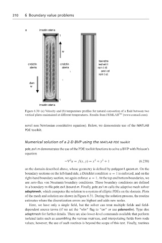
Figure 6.30 (a) Velocity and (b) temperature profiles for natural convection of a fluid between two
vertical plates maintained at different temperatures. Results from FEMLAB TM (www.comsol.com).

novel non Newtonian constitutive equation). Below, we demonstrate use of the MATLAB
PDE toolkit.

Numerical solution of a 2-D BVP using the MATLAB PDE toolkit
pde ex1.m demonstrates the use of the PDE toolkit functions to solve a BVP with Poisson’s
equation
2
2
2
−∇ u = f (x, y) = x + y + 1 (6.230)
on the domain described above, whose geometry is defined by polygon1 geom.m.Onthe
boundary sections on the left-hand side, a Dirichlet condition u = 1 is enforced, and on the
right-hand boundary section, we again enforce u = 1. At the top and bottom boundaries, we
use zero-flux von Neumann boundary conditions. These boundary conditions are defined
in a boundary m-file pde ex1 bound.m. Finally, pde ex1.m calls the adaptive mesh solver
adaptmesh, which computes the solution to a system of elliptic PDEs on the domain. Plots
of the mesh and solution are shown in Figure 6.31. During the solution process, the routine
estimates where the discretization errors are highest and adds new nodes.
Here, we have only a single field, but the solver can treat multiple fields and field-
dependent source terms (if we set the “nlin” flag to “on” or use pdenonlin). Type doc
adaptmesh for further details. There are also lower-level commands available that perform
isolated tasks such as assembling the various matrices, and interpolating fields from node
values; however, the use of such routines is beyond the scope of this text. Finally, routines