Page 316 - Numerical Methods for Chemical Engineering

The finite element method 305

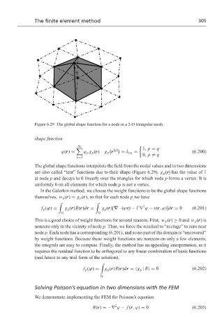
Figure 6.29 The global shape function for a node in a 2-D triangular mesh.

shape function
N n
1, p = q
[q]
ϕ(r) = ϕ p χ p (r) χ p r = δ pq = (6.200)
0, p = q
p=1
The global shape functions interpolate the field from the nodal values and in two dimensions
are also called “tent” functions due to their shape (Figure 6.29). χ p (r) has the value of 1
at node p and decays to 0 linearly over the triangles for which node p forms a vertex. It is
uniformly 0 on all elements for which node p is not a vertex.
In the Galerkin method, we choose the weight functions to be the global shape functions
themselves, w p (r) = χ p (r), so that for each node p we have
' '
2
f p (ϕ) = χ p (r)R(r)dr = χ p (r)[∇ · (ϕv) − ∇ ϕ − s(r,ϕ)]dr = 0 (6.201)

This is a good choice of weight functions for several reasons. First, w p (r) ≥ 0 and w p (r)is
nonzero only in the vicinity of node p. Thus, we force the residual to “average” to zero near
node p. Each node has a corresponding (6.201), and so no part of the domain is “uncovered”
by weight functions. Because these weight functions are nonzero on only a few elements,
the integrals are easy to compute. Finally, the method has an appealing interpretation, as it
requires the residual function to be orthogonal to any linear combination of basis functions
(and hence to any trial form of the solution),
'
f p (ϕ) = χ p (r)R(r)dr = χ p | R = 0 (6.202)

Solving Poisson’s equation in two dimensions with the FEM

We demonstrate implementing the FEM for Poisson’s equation
2
R(r) =−∇ ϕ − f (r,ϕ) = 0 (6.203)