Page 313 - Numerical Methods for Chemical Engineering

302 6 Boundary value problems

2

2

1

1

1 1 2 2
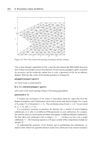
Figure 6.28 Plot of the initial mesh topology for polygon domain example.

This is done through a geometry m-file, a data file that informs the PDE toolkit functions
how to draw the boundary curves of the domain. For this system, polygon1 geom.m defines
the geometry, and its comments explain how to write a geometry m-file for an arbitrary
domain. With this file, a plot of the domain geometry is returned by
pdegplot(‘polygon1 geom’);
An initial mesh is constructed by

[P, E, T] = initmesh(‘polygon1 geom’);
with a plot of the mesh topology (Figure 6.28) being generated by

pdemesh(P, E, T);
P contains the coordinates of the nodes, E information about the edges that form the
domain boundaries, and T information about which nodes form which triangle. For a mesh
of N p nodes, P is of dimension 2 × N p . The coordinates of each node n ∈ [1, N p ] are stored
as x n = P 1n and y n = P 2n .
It is sometimes necessary to partition the domain into a number of nonoverlapping
subdomains, to be able to set different PDE parameters in each subdomain. For example,
this must be done in a heat transfer problem with regions of different thermal conductivity.
We then label each subdomain with an integer 1, 2,...,but here, we have only a single
subdomain “1.” All remaining regions in 2-D space outside of the computation domain are
labeled “0.”
To understand the geometry of the domain, and its partitioning into subdomains, we
need to know which line segments between nodes form either part of an external boundary