Page 310 - Numerical Methods for Chemical Engineering

The finite element method 299

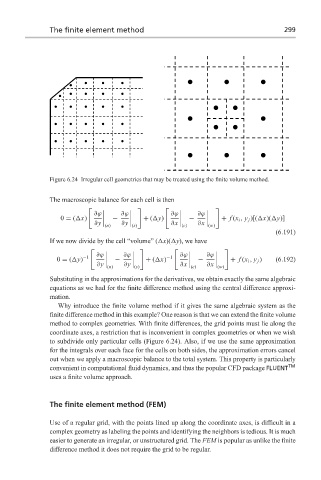
Figure 6.24 Irregular cell geometries that may be treated using the finite volume method.

The macroscopic balance for each cell is then

∂ϕ ∂ϕ ∂ϕ ∂ϕ
0 = ( x) − + ( y) − + f (x i , y j )[( x)( y)]
∂y (n) ∂y (s) ∂x (e) ∂x (w)
(6.191)
If we now divide by the cell “volume” ( x)( y), we have

0 = ( y) −1 ∂ϕ − ∂ϕ + ( x) −1 ∂ϕ − ∂ϕ + f (x i , y j ) (6.192)
∂y (n) ∂y (s) ∂x (e) ∂x (w)
Substituting in the approximations for the derivatives, we obtain exactly the same algebraic
equations as we had for the finite difference method using the central difference approxi-
mation.
Why introduce the finite volume method if it gives the same algebraic system as the
finite difference method in this example? One reason is that we can extend the finite volume
method to complex geometries. With finite differences, the grid points must lie along the
coordinate axes, a restriction that is inconvenient in complex geometries or when we wish
to subdivide only particular cells (Figure 6.24). Also, if we use the same approximation
for the integrals over each face for the cells on both sides, the approximation errors cancel
out when we apply a macroscopic balance to the total system. This property is particularly
convenient in computational fluid dynamics, and thus the popular CFD package FLUENT TM
uses a finite volume approach.

The finite element method (FEM)

Use of a regular grid, with the points lined up along the coordinate axes, is difficult in a
complex geometry as labeling the points and identifying the neighbors is tedious. It is much
easier to generate an irregular, or unstructured grid. The FEM is popular as unlike the finite
difference method it does not require the grid to be regular.