Page 309 - Numerical Methods for Chemical Engineering

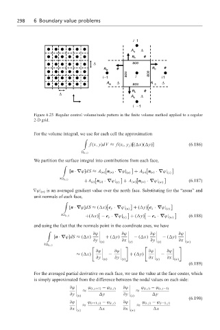
298 6 Boundary value problems

i 1

A n ∆
n n e
∆ ace
n w e n e e
ace ace
i −1 i i 1
A w ∆ ace A e ∆

∆ n s e
A s ∆
i −1
Figure 6.23 Regular control volume/node pattern in the finite volume method applied to a regular
2-D grid.

For the volume integral, we use for each cell the approximation
'
f (x, y)dV ≈ f (x i , y j )[( x)( y)] (6.186)
(i, j)
We partition the surface integral into contributions from each face,
'

[n · ∇ϕ]dS ≈ A (n) n (n) · ∇ϕ| + A (e) n (e) · ∇ϕ|
(n) (e)
∂ (i, j)
+A (s) n (s) · ∇ϕ| (s) + A (w) n (w) · ∇ϕ| (w) (6.187)
∇ϕ| (n) is an averaged gradient value over the north face. Substituting for the “areas” and
unit normals of each face,
'

[n · ∇ϕ]dS ≈ ( x) e y · ∇ϕ| (n) + ( y) e x · ∇ϕ| (e)

∂ (i, j)
+( x) − e y · ∇ϕ| (s) + ( y) − e x · ∇ϕ| (w) (6.188)
and using the fact that the normals point in the coordinate axes, we have

'
∂ϕ ∂ϕ ∂ϕ ∂ϕ
[n · ∇ϕ]dS ≈ ( x) + ( y) − ( x) − ( y)
∂y ∂x ∂y ∂x
(n) (e) (s) (w)
∂ (i, j)

∂ϕ ∂ϕ ∂ϕ ∂ϕ
≈ ( x) − + ( y) −
∂y ∂y ∂x ∂x
(n) (s) (e) (w)
(6.189)
For the averaged partial derivative on each face, we use the value at the face center, which
is simply approximated from the difference between the nodal values on each side:

∂ϕ ϕ (i, j+1) − ϕ (i, j) ∂ϕ ϕ (i, j) − ϕ (i, j−1)
≈ ≈
∂y y ∂y y
(n) (s)
(6.190)

∂ϕ ϕ (i+1, j) − ϕ (i, j) ∂ϕ ϕ (i, j) − ϕ (i−1, j)
≈ ≈
∂x x ∂x x
(e) (w)