Page 367 - Numerical Methods for Chemical Engineering

356 7 Probability theory and stochastic simulation

= 1
e
= 1
saes
sain re = 1
∆ a = 1
2
2
1

1

−

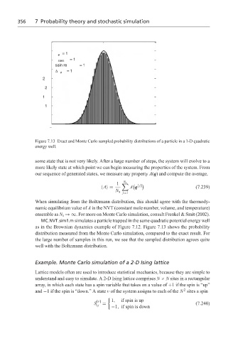
Figure 7.13 Exact and Monte Carlo sampled probability distributions of a particle in a 1-D quadratic
energy well.

some state that is not very likely. After a large number of steps, the system will evolve to a
more likely state at which point we can begin measuring the properties of the system. From
our sequence of generated states, we measure any property A(q) and compute the average,
1 [ j]
N s
A = A q (7.239)
N s
j=1
When simulating from the Boltzmann distribution, this should agree with the thermody-
namic equilibrium value of A in the NVT (constant mole number, volume, and temperature)
ensemble as N s →∞. For more on Monte Carlo simulation, consult Frenkel & Smit (2002).
MC NVT sim1.m simulates a particle trapped in the same quadratic potential energy well
as in the Brownian dynamics example of Figure 7.12. Figure 7.13 shows the probability
distribution measured from the Monte Carlo simulation, compared to the exact result. For
the large number of samples in this run, we see that the sampled distribution agrees quite
well with the Boltzmann distribution.

Example. Monte Carlo simulation of a 2-D Ising lattice
Lattice models often are used to introduce statistical mechanics, because they are simple to
understand and easy to simulate. A 2-D Ising lattice comprises N × N sites in a rectangular
array, in which each state has a spin variable that takes on a value of +1 if the spin is “up”
2
and −1 if the spin is “down.” A state ν of the system assigns to each of the N sites a spin

[ν] 1, if spin is up
S = (7.240)
ij −1, if spin is down