Page 398 - Numerical Methods for Chemical Engineering

The Bayesian view of statistical inference 387

after having conducted both sets of experiments is

1
p θ|y , y 2 ∝ l 2 θ|y 2 p θ|y 1 (8.67)
Bayes’ theorem provides a framework for learning from new experiences.

Finally, in some instances we may wish to use a prior based upon past experience with
similar systems. While such priors violate the ideal of objectivity in statistical analysis, they
can provide better estimates if the subjective prior is chosen well (i.e., the “expert” choosing
the prior knows what he is talking about). Several approaches to constructing priors to agree
with preexisting conditions, data, or experience are discussed in Robert, (2001).
Here, we consider a method for generating priors that is “objective” in the sense that
as long as different analysts agree to use this approach, they will independently come to
(nearly) the same statistical conclusions given only the predictors, response data, model, and
likelihood function. The basic technique, discussed below, is to identify a data-translation,
or symmetry, property that the likelihood function has, and choose the prior so that the
posterior density retains the same property. Such a prior does not give undue emphasis to
any particular region of parameter space and thus is said to be noninformative. As we later
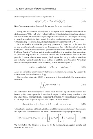
show, for the single-response likelihood (8.64), a noninformative prior is

p(θ,σ) = p(θ)p(σ) p(θ) ∼ c p(σ) ∝ σ −1 (8.68)

As we use a prior that is uniform in θ, the Bayesian most probable estimate θ M agrees with
the maximum likelihood estimate θ MLE .
The noninformative prior (8.68) is improper as it does not satisfy the normalization
condition
' '
p(θ,σ)dσdθ = 1 (8.69)
σ>0
P
and furthermore does not integrate to a finite value. For some aspects of our analysis, this
is not a problem as the posterior density is still proper, but when testing hypotheses, it is
important that the prior density also be a proper distribution. We suggest here a very simple
fix to this problem, by providing the a priori upper and lower bounds,

θ ={θ|θ j,lo ≤ θ j ≤ θ j,hi , j = 1, 2,..., N} σ lo ≤ σ ≤ σ hi (8.70)

withindicatorfunctions I θ (θ)and I σ (σ)thatequal1forparametersthatsatisfythesebounds
and equal 0 for values outside of the bounds. We then define the proper prior density
   
' '
p(θ,σ) = c 0 σ −1 I θ (θ)I σ (σ) c −1 =  I θ (θ)dθ   σ −1 I σ (σ)dσ  (8.71)
0
P σ>0

We show below why this prior is used, but for the moment, let us accept it as valid and
continue our discussion.