Page 396 - Numerical Methods for Chemical Engineering

The Bayesian view of statistical inference 385

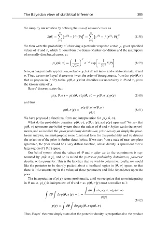
We simplify our notation by defining the sum of squared errors as
N 2 N 2
[k]
[k]

S(θ) = y [k] − ˆ y (θ) = y [k] − f x ; θ (8.58)
k=1 k=1
We then write the probability of observing a particular response vector y, given specified
values of θ and σ, which follows from the Gauss–Markov conditions and the assumption
of normally-distributed errors, as
N
1 −N 1

p(y|θ,σ) = √ σ exp − 2 S(θ) (8.59)
2π 2σ
Now, in our particular application, we know y, but do not know, and wish to estimate, θ and
σ. Thus, we turn to Bayes’ theorem to invert the order of the arguments, from the p(y|θ,σ)
that we propose in (8.59), to the p(θ,σ|y) that describes our uncertainty in θ and σ,given
the known value of y.
Bayes’ theorem states that
p(y, θ,σ) = p(y|θ,σ)p(θ,σ) = p(θ,σ|y)p(y) (8.60)

and thus
p(y|θ,σ)p(θ,σ)
p(θ,σ|y) = (8.61)
p(y)
We have proposed a functional form and interpretation for p(y|θ,σ).
What do the probability densities p(θ,σ), p(θ,σ|y), and p(y) represent? We say that
p(θ,σ) represents our belief system about the values of θ and σ before we do the experi-
ments, and so is called the prior probability distribution, prior density, or simply the prior.
In our analysis, we must propose some functional form for this probability, and we discuss
the selection of the prior in further detail below. If we start from a state of near-complete
ignorance, the prior should be a very diffuse function, whose density is spread out over a
large region of ( θ,σ) space.
Our belief system about the values of θ and σ after we do the experiments is rep-
resented by p(θ,σ|y), and so is called the posterior probability distribution, posterior
density,orthe posterior. This is the function that we wish to determine. Ideally, we would
like the posterior to be sharply peaked about a localized region in (θ, σ) space, so that
there is little uncertainty in the values of these parameters and little dependence upon the
prior.
The interpretation of p( y) seems problematic, until we recognize that upon integrating
in θ and σ, p( y) is independent of θ and σ as p(θ,σ|y) must normalize to 1:
' '
dθ dσ p(y|θ,σ)p(θ,σ)
' '
dθ dσ p(θ,σ|y) = 1 =
p(y)
(8.62)
' '
p(y) = dθ dσ p(y|θ,σ)p(θ,σ)

Thus, Bayes’ theorem simply states that the posterior density is proportional to the product