Page 392 - Numerical Methods for Chemical Engineering

The Bayesian view of statistical inference 381

and find that θ 2, lo > 0, then the data suggest that the difference in means between the two
subsets is statistically significant; i.e., it is probably not due solely to random error.
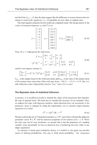
The least-squares estimates for this model are computed easily. The design matrix X, the
T
vector of measured responses y, and X y are
   
10 121.9
 10   113.4 
   
   
 10   112.2 

    934.3
T
 10   106.1 
X y = (8.39)
480.7
X =   y =  
 11   120.7 
   
 11   119.5 
   
 11   116.5 
11 124.0
Thus, for n = 4 data points for each strain,

(2n) n 84
T
X X = =
n n 44
(8.40)
−1 −1
T −1 n −n 0.25 −0.25
X X = −1 −1 =
−n (2n ) −0.25 0.5
and the least-squares estimate is

θ LS, 1 T −1 T 0.25 −0.25 934.3 113.4
= (X X) X y = = (8.41)
θ LS, 2 0.25 0.5 480.7 6.7750
θ LS, 1 is the sample mean for the wild-type strain, and θ LS, 2 is the value of the sample mean
of the mutant strain minus that of the wild-type strain, 120.16 − 113.41 = 6.75. But, is it
still within the realm of plausibility that the “true” value of θ 2 is zero?
The Bayesian view of statistical inference

In practice, it is insufficient merely to identify the values of the parameters that minimize
the sum of squared errors. We need also to consider the accuracy of our estimates. Here,
we address this topic with Bayesian statistics, which describes how our uncertainty in the
parameter values is changed by doing the experiments. Let us consider single-response
regression of a model
[k]

y [k] = f x ; θ + ε [k] (8.42)
N
We have a particular set of N measured responses y ∈ , and wish to estimate the unknown
P
parameter vector θ ∈ and the statistical properties of the random error ε ∈ . While
the error may not be truly stochastic, we assume that it has the properties of a random
variable, since presumably we have no practical way of predicting the error value in any
single experiment.
As statistics is based upon probability theory, it is helpful to cite again two possible
means of defining probabilities. One way to think about probability – the frequentist