Page 387 - Numerical Methods for Chemical Engineering

376 8 Bayesian statistics and parameter estimation

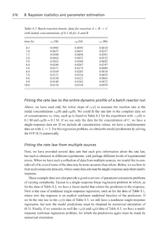
Table 8.3 Batch reaction kinetic data for reaction A + B → C
with initial concentrations of 0.1 M for A and B

time (h) c A (M) c B (M) c C (M)
0.5 0.0985 0.0995 0.0010
1.0 0.0637 0.0651 0.0357
1.5 0.0500 0.0496 0.0501
2.0 0.0462 0.0453 0.0512
3.0 0.0363 0.0384 0.0682
4.0 0.0248 0.0247 0.0747
5.0 0.0171 0.0174 0.0809
6.0 0.0168 0.0203 0.0818
7.0 0.0131 0.0136 0.0858
8.0 0.0150 0.0121 0.0863
9.0 0.0140 0.0142 0.0872
10.0 0.0134 0.0134 0.0928

Fitting the rate law to the entire dynamic profile of a batch reactor run

Above, we have used only the initial slope of c C (t) to measure the reaction rate at the
initial concentrations c A (0) and c B (0). We could fit the rate law to the complete data set
of concentrations vs. time, such as is found in Table 8.3 for the experiment with c A (0) =
0.1 M and c B (0) = 0.1 M. If we use only the data for the concentration of C, we have a
single-response data set. If we include all concentration values, we have a multiresponse
data set with L = 3. For this regression problem, we obtain the model predictions by solving
the IVP (8.5) numerically.

Fitting the rate law from multiple sources
Here, we have provided several data sets that each give information about the rate law,
but each is obtained in different experiments, with perhaps different levels of experimental
errors. When we have such a collection of data from multiple sources, we would like to con-
sider all of it, even if some of the data may be more accurate than others. Below, we see how to
treatsuchcompositedatasets,wheresomedatasetsmaybesingle-responseandothersmulti-
response.
These example data sets also provide a good overview of parameter estimation problems
of varying complexity. Easiest is a single-response linear regression problem in which, as
for the data of Table 8.2, we have a linear model that relates the predictors to the response.
Next is the case of nonlinear single-response regression, such as for the data of Table 8.1,
where now the response is an explicit nonlinear analytical function of the predictors. If
we fit the rate law to the c C (t) data of Table 8.3, we still have a nonlinear single-response
regression, but now the model predictions must be obtained by numerical simulation of
(8.5). Finally, if we consider as well the c A (t) and c B (t) data of Table 8.3, we have a multi-
response nonlinear regression problem, for which the predictions again must be made by
numerical simulation.