Page 382 - Numerical Methods for Chemical Engineering

Problems 371

0 the “start” values of the participating monomer units. At each 0.05 increment of the acid
conversion, plot the chain length distribution, up to near the gel point. Unless the number
of monomers that you simulate is very large, the simulation will not be accurate near the
gel point. Plot the measured DP w as a function of conversion, and compare to the previous
analytical result.

N
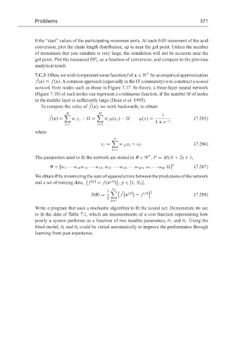
7.C.3.Often,wewishtorepresentsomefunctionfof x ∈ byanempiricalapproximation
˜
f (x) ≈ f (x). A common approach (especially in the IT community) is to construct a neural
network from nodes such as those in Figure 7.17. In theory, a three-layer neural network
(Figure 7.18) of such nodes can represent a continuous function, if the number M of nodes
in the middle layer is sufficiently large (Dean et al. 1995).
˜
To compute the value of f (x), we work backwards, to obtain
M M
1
˜
f (x) = w j t j − = w j ϕ(s j ) − ϕ(x) = (7.285)
1 + e −x
j=1 j=1
where
N

s j = w jk x k − ω j (7.286)
k=1
P
The parameters used to fit the network are stored in θ ∈ , P = M(N + 2) + 1,
θ = [w 1 ··· w M w 11 ··· w 1N w 21 ··· w 2N ··· w MN ω 1 ··· ω M ] T (7.287)
We obtain θ by minimizing the sum of squared errors between the predictions of the network
[p] [p]
and a set of training data, f = f (x ) , p ∈ [1, N d ],
N d
1 [p] [p] 2
˜

S(θ) = f x − f (7.288)
2
p=1
Write a program that uses a stochastic algorithm to fit the neural net. Demonstrate its use
to fit the data of Table 7.1, which are measurements of a cost function representing how
poorly a system performs as a function of two tunable parameters, θ 1 and θ 2 . Using the
fitted model, θ 1 and θ 2 could be varied automatically to improve the performance through
learning from past experience.