Page 381 - Numerical Methods for Chemical Engineering

370 7 Probability theory and stochastic simulation

Table 7.1 Measured data of system
performance

θ 1 θ 2 F(θ)
2.653 2.639 0.948
2.625 2.703 0.744
1.865 2.699 0.381
2.591 3.104 0.393
1.337 2.772 0.648
1.779 2.699 0.411
2.470 2.515 1.162
1.265 3.247 0.784

s 1 t 1
w Σ w
1 11 1

w 12 ω 1
−1
w 1
w t
1 1
w 21
s t 2
2 2
Σ w 2
w 22 w t ∼
2 2
f
ω 2
w 2 Σ
−1
Ω
w 1 −1
wt
w 2 s t
Σ w
w ω
−1
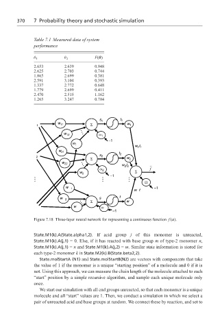
Figure 7.18 Three-layer neural network for representing a continuous function f (x).

State.M1(k).A(State.alpha1,2). If acid group j of this monomer is unreacted,
State.M1(k).A(j,1) = 0. Else, if it has reacted with base group m of type-2 monomer n,
State.M1(k).A(j,1) = n and State.M1(k).A(j,2) = m. Similar state information is stored for
each type-2 monomer k in State.M2(k).B(State.beta2,2).
State.molStartA (N1) and State.molStartB(N2) are vectors with components that take
the value of 1 if the monomer is a unique “starting position” of a molecule and 0 if it is
not. Using this approach, we can measure the chain length of the molecule attached to each
“start” position by a simple recursive algorithm, and sample each unique molecule only
once.
We start our simulation with all end groups unreacted, so that each monomer is a unique
molecule and all “start” values are 1. Then, we conduct a simulation in which we select a
pair of unreacted acid and base groups at random. We connect these by reaction, and set to