Page 386 - Numerical Methods for Chemical Engineering

Fitting kinetic parameters of a chemical reaction 375

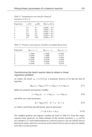
Table 8.1 Instantaneous rate data for chemical
reaction A + B → C

Experiment c A (M) c B (M) Rate r R1 (M/s)
1 0.1 0.1 0.0246 × 10 −3
2 0.2 0.1 0.0483 × 10 −3
3 0.1 0.2 0.0501 × 10 −3
4 0.2 0.2 0.1003 × 10 −3
5 0.05 0.2 0.0239 × 10 −3
6 0.2 0.05 0.0262 × 10 −3

Table 8.2 Predictor and response variables in modified linear form

Experiment log c A = x 1 log c B = x 2 log r R1 = y
10
10
10
1 −1.0000 −1.0000 −4.6096
2 −0.6990 −1.0000 −4.3157
3 −1.0000 −0.6990 −4.2999
4 −0.6990 −0.6990 −3.9988
5 −1.3010 −0.6990 −4.6224
6 −0.6990 −1.3010 −4.5818

Transforming the batch reactor data to obtain a linear
regression problem

As written, the model r R1 = k 1 (T )c c is nonlinear; however, if we take the base-10
v a v b
A B
logarithm,
(8.7)
log r R1 = log k 1 (T ) + ν a log c A + ν b log c B
10
10
10
10
define new predictor and response variables
y = log r R1 x 1 = log c A x 2 = log c B (8.8)
10 10 10
and define new model parameters
β 0 = log k 1 (T ) β 1 = ν a β 2 = ν b (8.9)
10
we obtain a model that depends linearly upon its parameters:

y = β 0 + β 1 x 1 + β 2 x 2 (8.10)
The modified predictor and response variables are listed in Table 8.2. From this single-
response linear regression, we obtain estimates for the reaction exponents ν a , ν b , and the
rate constant k 1 (T). Such transformations are common in practice, but care must be taken in
drawing the proper statistical conclusions as the transformations also act upon the random
noise that is assumed present.