Page 388 - Numerical Methods for Chemical Engineering

Single-response linear regression 377

Single-response linear regression

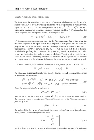
We first discuss the regression, or estimation, of parameters in linear models from single-
response data. Let us say that we have performed a set of N experiments in which for each
[k] [k] [k]
experiment k = 1, 2,..., N, the set of predictor variables {x , x ,..., x } is known a
1 2 M
[k]
priori, and a measurement is made of the single-response variable y . We assume that this
single-response variable depends linearly upon the predictors,
y [k] = β 0 + β 1 x [k] + β 2 x [k] +· · · + β M x [k] + ε [k] (8.11)
1 2 M
ε [k] is some random measurement error for the kth experiment. Due to this error, the
measured response is not equal to the “true” response of the system, and the statistical
properties of the error are very important, although generally unknown at the time of
measurement. The “true” parameters {β 0 ,β 1 ,...,β M } are those that describe the sys-
tem behavior perfectly in the absence of any random, model, or predictor error. That
is, we hypothesize that the model is indeed a valid one. Thus, the set of predictor vari-
ables chosen indeed completely specifies the response of the system (in the absence
of random error) and the relationship between the response and each predictor is truly
linear.
In some instances, we wish to fit a model with a zero y-intercept β 0 = 0, such that
y [k] = β 1 x 1 [k] + β 2 x 2 [k] +· · · + β M x [k] + ε [k] (8.12)
M
We introduce a common notation for both cases by defining for each experiment the vectors
of predictors and parameters,

x [k] = 1 x [k] x [k] ... x [k] θ = [β 0 β 1 β 2 ...β M ] T with y-intercept
1 2 M
(8.13)

x [k] = x [k] x [k] ... x [k] θ = [β 1 β 2 ...β M ] T without y-intercept
1 2 M
Then, the response in the kth experiment is
y [k] = x [k] · θ (true) + ε [k] (8.14)

Because we do not know the “true” values θ (true) of the parameters, we must consider
the parameter vector to be adjustable. The predicted response in the kth experiment, as a
function of θ,is
[k]
ˆ y (θ) = x [k] · θ (8.15)
We further define for our set of experiments the design matrix X to contain for each exper-
iment, the row vector of the predictor values,
 [1] 
— x —
 — x [2] 

. —  (8.16)
X =  . 
 . 
— x [N] —
For dim(θ) = P, X is an N × P matrix. X is specified when we design the set of experiments