Page 391 - Numerical Methods for Chemical Engineering

380 8 Bayesian statistics and parameter estimation

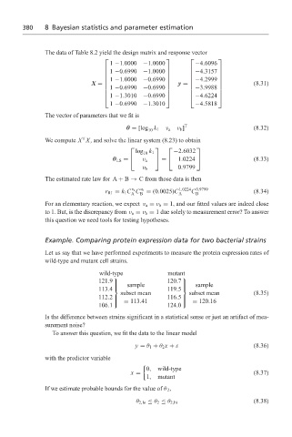
The data of Table 8.2 yield the design matrix and response vector
   
1 −1.0000 −1.0000 −4.6096
 1 −0.6990 −1.0000   


 −4.3157 
 1 −1.0000   

(8.31)
−0.6990 
 −4.2999 
 1 −0.6990 −0.6990  y =  

X = 
 −3.9988 

 1 −1.3010   
−0.6990   −4.6224 
1 −0.6990 −1.3010 −4.5818
The vector of parameters that we fit is
θ = [log k 1 ν a ν b ] T (8.32)
10
T
We compute X X, and solve the linear system (8.23) to obtain
   
log k 1 −2.6032
10
θ LS =  ν a  =  1.0224  (8.33)
0.9799
ν b
The estimated rate law for A + B → C from those data is then
v a
r R1 = k 1 C C v b = (0.0025)C 1.0224 C 0.9799 (8.34)
A B A B
For an elementary reaction, we expect ν a = ν b = 1, and our fitted values are indeed close
to 1. But, is the discrepancy from ν a = ν b = 1 due solely to measurement error? To answer
this question we need tools for testing hypotheses.
Example. Comparing protein expression data for two bacterial strains
Let us say that we have performed experiments to measure the protein expression rates of
wild-type and mutant cell strains.
wild-type mutant
 
sample 120.7  sample
121.9 
 
113.4  119.5 
subset mean subset mean (8.35)
 = 113.41  = 120.16
112.2  116.5 


106.1 124.0
Is the difference between strains significant in a statistical sense or just an artifact of mea-
surement noise?
To answer this question, we fit the data to the linear model
y = θ 1 + θ 2 x + ε (8.36)
with the predictor variable

0, wild-type
x = (8.37)
1, mutant
If we estimate probable bounds for the value of θ 2 ,

(8.38)
θ 2,lo ≤ θ 2 ≤ θ 2,hi