Page 384 - Numerical Methods for Chemical Engineering

Fitting kinetic parameters of a chemical reaction 373

easred
[k]
x [k] x ∈ℜ M ˆ y (θ) y [k]
Model of system − resnses
ied int redict predicted y (r) ∈ℜ L r eac
predictor sste resnses responses eerient
variables in eac eerient r eac
[k]
r eac r x and θ eerient
eerient
[k]
[k]
k = 1, 2, ..., N ˆ y (θ) = f(x ; θ) var araeters θ t
iniie disareeent
θ ∈ℜ P etween easred and
redicted resnses
adstae araeters
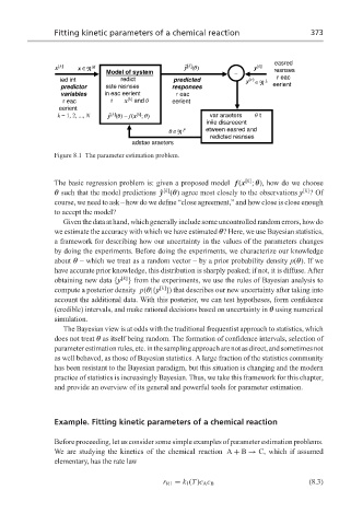
Figure 8.1 The parameter estimation problem.

[k]
The basic regression problem is: given a proposed model f (x ; θ), how do we choose
[k]
[k]
θ such that the model predictions ˆy (θ) agree most closely to the observations y ?Of
course, we need to ask – how do we define “close agreement,” and how close is close enough
to accept the model?
Given the data at hand, which generally include some uncontrolled random errors, how do
we estimate the accuracy with which we have estimated θ? Here, we use Bayesian statistics,
a framework for describing how our uncertainty in the values of the parameters changes
by doing the experiments. Before doing the experiments, we characterize our knowledge
about θ – which we treat as a random vector – by a prior probability density p(θ). If we
have accurate prior knowledge, this distribution is sharply peaked; if not, it is diffuse. After
[k]
obtaining new data {y } from the experiments, we use the rules of Bayesian analysis to
[k]
compute a posterior density p(θ|{y }) that describes our new uncertainty after taking into
account the additional data. With this posterior, we can test hypotheses, form confidence
(credible) intervals, and make rational decisions based on uncertainty in θ using numerical
simulation.
The Bayesian view is at odds with the traditional frequentist approach to statistics, which
does not treat θ as itself being random. The formation of confidence intervals, selection of
parameterestimationrules,etc.inthesamplingapproacharenotasdirect,andsometimesnot
as well behaved, as those of Bayesian statistics. A large fraction of the statistics community
has been resistant to the Bayesian paradigm, but this situation is changing and the modern
practice of statistics is increasingly Bayesian. Thus, we take this framework for this chapter,
and provide an overview of its general and powerful tools for parameter estimation.

Example. Fitting kinetic parameters of a chemical reaction

Before proceeding, let us consider some simple examples of parameter estimation problems.
We are studying the kinetics of the chemical reaction A + B → C, which if assumed
elementary, has the rate law

(8.3)
r R1 = k 1 (T )c A c B