Page 380 - Numerical Methods for Chemical Engineering

Problems 369

1
n
2 Σ Σ = 1

n

w 1
ϕ −
1 e
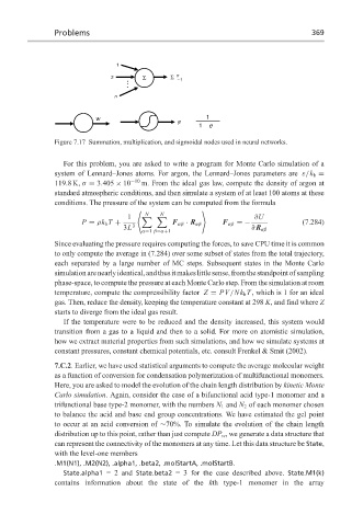
Figure 7.17 Summation, multiplication, and sigmoidal nodes used in neural networks.

For this problem, you are asked to write a program for Monte Carlo simulation of a
system of Lennard–Jones atoms. For argon, the Lennard–Jones parameters are ε/k b =
119.8K,σ = 3.405 × 10 −10 m. From the ideal gas law, compute the density of argon at
standard atmospheric conditions, and then simulate a system of at least 100 atoms at these
conditions. The pressure of the system can be computed from the formula
7 N N 8
1 ∂U
P = ρk b T + 3 F αβ · R αβ F αβ =− (7.284)
3L ∂ R αβ
α=1 β=α+1
Since evaluating the pressure requires computing the forces, to save CPU time it is common
to only compute the average in (7.284) over some subset of states from the total trajectory,
each separated by a large number of MC steps. Subsequent states in the Monte Carlo
simulationarenearlyidentical,andthusitmakeslittlesense, fromthestandpointofsampling
phase-space, to compute the pressure at each Monte Carlo step. From the simulation at room
temperature, compute the compressibility factor Z = PV/Nk b T , which is 1 for an ideal
gas. Then, reduce the density, keeping the temperature constant at 298 K, and find where Z
starts to diverge from the ideal gas result.
If the temperature were to be reduced and the density increased, this system would
transition from a gas to a liquid and then to a solid. For more on atomistic simulation,
how we extract material properties from such simulations, and how we simulate systems at
constant pressures, constant chemical potentials, etc. consult Frenkel & Smit (2002).
7.C.2. Earlier, we have used statistical arguments to compute the average molecular weight
as a function of conversion for condensation polymerization of multifunctional monomers.
Here, you are asked to model the evolution of the chain length distribution by kinetic Monte
Carlo simulation. Again, consider the case of a bifunctional acid type-1 monomer and a
trifunctional base type-2 monomer, with the numbers N 1 and N 2 of each monomer chosen
to balance the acid and base end group concentrations. We have estimated the gel point
to occur at an acid conversion of ∼70%. To simulate the evolution of the chain length
distribution up to this point, rather than just compute DP w , we generate a data structure that
can represent the connectivity of the monomers at any time. Let this data structure be State,
with the level-one members
.M1(N1), .M2(N2), .alpha1, .beta2, .molStartA, .molStartB.
State.alpha1 = 2 and State.beta2 = 3 for the case described above. State.M1(k)
contains information about the state of the kth type-1 monomer in the array