Page 403 - Numerical Methods for Chemical Engineering

392 8 Bayesian statistics and parameter estimation

1

µσ

2

1
−2 −1 1 2
µ
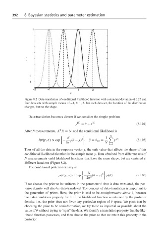
Figure 8.2 Data-translation of conditional likelihood function with a standard deviation of 0.25 and
four data sets with sample means of −1, 0, 1, 2. For each data set, the location of the distribution
changes, but not the shape.

Data-translation becomes clearer if we consider the simple problem

y [k] = θ + ε [k] (8.104)
T
After N measurements, X X = N, and the conditional likelihood is
1 N
N 2 1 [k]
l(θ|y,σ) ∝ exp − (θ − ¯ y) ¯ y = θ LS = y (8.105)
2σ 2 N
k=1
Thus of all the data in the response vector y, the only value that affects the shape of this
conditional likelihood function is the sample mean ¯ y. Data obtained from different sets of
N measurements yield likelihood functions that have the same shape, but are centered at
different locations (Figure 8.2).
The conditional posterior density is
1
N 2
p(θ|y,σ) ∝ exp − (θ − ¯ y) p(θ) (8.106)
2σ 2
If we choose the prior to be uniform in the parameter θ that is data-translated, the pos-
terior density will also be data-translated. The concept of data-translation is important to
the generation of priors. Here, the prior is said to be noninformative about θ, because
the data-translation property for θ of the likelihood function is retained by the posterior
density; i.e., the prior does not favor any particular region of θ-space. We posit that by
choosing the prior to be noninformative, we try to be as impartial as possible about the
value of θ without trying to “spin” the data. We identify a translation property that the like-
lihood function possesses, and then choose the prior so that we retain this property in the
posterior.