Page 407 - Numerical Methods for Chemical Engineering

396 8 Bayesian statistics and parameter estimation

ν 2 ν

2 2

1 1

− −

ν 1 ν 2

2 2

1 1

− −

2
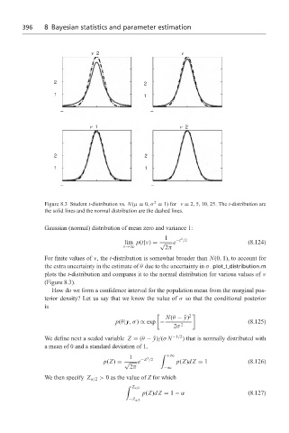
Figure 8.3 Student t-distribution vs. N(µ = 0,σ = 1) for v = 2, 5, 10, 25. The t-distribution are
the solid lines and the normal distribution are the dashed lines.

Gaussian (normal) distribution of mean zero and variance 1:
1 −t /2
2
lim p(t|ν) = √ e (8.124)
ν→∞ 2π
For finite values of ν, the t-distribution is somewhat broader than N(0, 1), to account for
the extra uncertainty in the estimate of θ due to the uncertainty in σ. plot t distribution.m
plots the t-distribution and compares it to the normal distribution for various values of ν
(Figure 8.3).
How do we form a confidence interval for the population mean from the marginal pos-
terior density? Let us say that we know the value of σ so that the conditional posterior
is

N(θ − ¯ y)
2
p(θ|y,σ) ∝ exp − 2 (8.125)
2σ
We define next a scaled variable Z = (θ − ¯ y)/(σ N −1/2 ) that is normally distributed with
a mean of 0 and a standard deviation of 1,

1 −Z /2 ' +∞
2
p(Z) = √ e p(Z)dZ = 1 (8.126)
2π −∞
We then specify Z α/2 > 0 as the value of Z for which
'
Z α/2
p(Z)dZ = 1 − α (8.127)
−Z α/2