Page 409 - Numerical Methods for Chemical Engineering

398 8 Bayesian statistics and parameter estimation

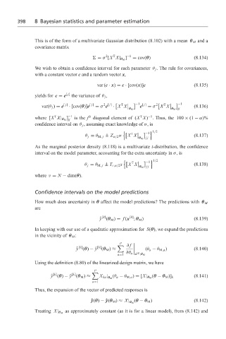
This is of the form of a multivariate Gaussian distribution (8.102) with a mean θ M and a
covariance matrix
2 T −1
= σ [X X| θ M ] = cov(θ) (8.134)
We wish to obtain a confidence interval for each parameter θ j . The rule for covariances,
with a constant vector c and a random vector x,

var (c · x) = c · [cov(x)]c (8.135)
yields for c = e [ j] the variance of θ j ,

2 [ j]

var(θ j ) = e [ j] · [cov(θ)]e [ j] = σ e · X X −1 [ j] = σ 2 X X −1 (8.136)
e
T
T
θ M θ M jj
T −1 th T −1
]
where [X X| θ M jj is the j diagonal element of (X X) . Thus, the 100 × (1 − α)%
confidence interval on θ j , assuming exact knowledge of σ,is
9 : 1/2
−1
θ j = θ M, j ± Z α/2 σ X X (8.137)
T
θ M jj
As the marginal posterior density (8.118) is a multivariate t-distribution, the confidence
interval on the model parameter, accounting for the extra uncertainty in σ,is
1/2
9 :
−1
θ j = θ M, j ± T ν,α/2 s X X (8.138)
T
θ M jj
where ν = N − dim(θ).
Confidence intervals on the model predictions
How much does uncertainty in θ affect the model predictions? The predictions with θ M
are
[k]
[k]
ˆ y (θ M ) = f (x ; θ M ) (8.139)
In keeping with our use of a quadratic approximation for S(θ), we expand the predictions
in the vicinity of θ M :
P

[k] [k] ∂ f
ˆ y (θ) − ˆ y (θ M ) ≈ (θ a − θ M,a ) (8.140)

[k]
a=1 ∂θ a x ;θ M
Using the definition (8.80) of the linearized design matrix, we have
P

[k] [k]
ˆ y (θ) − ˆ y (θ M ) ≈ X ka | (θ a − θ M,a ) = [X| θ M (θ − θ M )] k (8.141)
θ M
a=1
Thus, the expansion of the vector of predicted responses is
ˆ y(θ) − ˆy(θ M ) ≈ X| (θ − θ M ) (8.142)
θ M
as approximately constant (as it is for a linear model), from (8.142) and
Treating X| θ M