Page 413 - Numerical Methods for Chemical Engineering

402 8 Bayesian statistics and parameter estimation

0.0019 0.0031
0.9057 1.0946
0.9057 1.0946

Thus, the fitted rate law is
r R1 = (0.0025)c 1.0001 1.0001 (8.146)
c
A B
with the approximate 95% confidence intervals

0.0019 ≤ k 1 ≤ 0.0031 0.9057 ≤ ν a ≤ 1.0946 0.9057 ≤ ν b ≤ 1.0946 (8.147)
Therefore, the data do appear to be consistent with an elementary reaction. Below, we test
this hypothesis more rigorously using MCMC simulation with the exact posterior.

Example. Fitting the rate constant from the full curve of concentration
of C vs. time for a batch reactor experiment

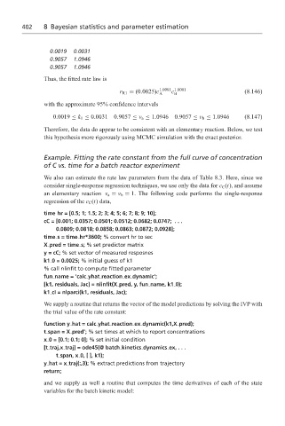
We also can estimate the rate law parameters from the data of Table 8.3. Here, since we
consider single-response regression techniques, we use only the data for c C (t), and assume
an elementary reaction ν a = ν b = 1. The following code performs the single-response
regression of the c C (t) data,
time hr = [0.5; 1; 1.5; 2; 3; 4; 5; 6; 7; 8; 9; 10];
cC = [0.001; 0.0357; 0.0501; 0.0512; 0.0682; 0.0747; . . .
0.0809; 0.0818; 0.0858; 0.0863; 0.0872; 0.0928];
time s = time hr*3600; % convert hr to sec
X pred = time s; % set predictor matrix
y = cC; % set vector of measured resposnes
k1 0 = 0.0025; % initial guess of k1
% call nlinfit to compute fitted parameter
fun name = ‘calc yhat reaction ex dynamic’;
[k1, residuals, Jac] = nlinfit(X pred, y, fun name, k1 0);
k1 cI = nlparci(k1, residuals, Jac);
We supply a routine that returns the vector of the model predictions by solving the IVP with
the trial value of the rate constant:
function y hat = calc yhat reaction ex dynamic(k1,X pred);
t span = X pred’; % set times at which to report concentrations
x 0 = [0.1; 0.1; 0]; % set initial condition
[t traj,x traj] = ode45(@ batch kinetics dynamics ex,...
t span, x 0, [ ], k1);
y hat=x traj(:,3); % extract predictions from trajectory
return;
and we supply as well a routine that computes the time derivatives of each of the state
variables for the batch kinetic model: