Page 415 - Numerical Methods for Chemical Engineering

404 8 Bayesian statistics and parameter estimation

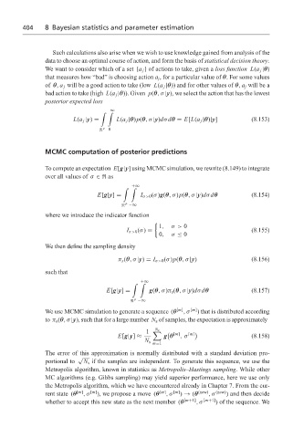
Such calculations also arise when we wish to use knowledge gained from analysis of the
data to choose an optimal course of action, and form the basis of statistical decision theory.
We want to consider which of a set {a j } of actions to take, given a loss function L(a j |θ)
that measures how “bad” is choosing action a j , for a particular value of θ. For some values
of θ, a j will be a good action to take (low L(a j |θ)) and for other values of θ, a j will be a
bad action to take (high L(a j |θ)). Given p(θ,σ|y), we select the action that has the lowest
posterior expected loss
∞
' '
L(a j |y) = L(a j |θ)p(θ,σ|y)dσdθ = E[L(a j |θ)|y] (8.153)
P 0

MCMC computation of posterior predictions

To compute an expectation E[g|y] using MCMC simulation, we rewrite (8.149) to integrate
over all values of σ ∈ as
+∞
' '
E[g|y] = I σ>0 (σ)g(θ,σ)p(θ,σ|y)dσdθ (8.154)
P
−∞
where we introduce the indicator function

1, σ > 0
I σ>0 (σ) = (8.155)
0, σ ≤ 0
We then define the sampling density
π s (θ,σ|y) = I σ>0 (σ)p(θ,σ|y) (8.156)

such that
+∞
' '
E[g|y] = g(θ,σ)π s (θ,σ|y)dσdθ (8.157)
P
−∞
We use MCMC simulation to generate a sequence (θ [m] ,σ [m] ) that is distributed according
to π s (θ,σ|y), such that for a large number N s of samples, the expectation is approximately

1 [m] [m]
N s
E[g|y] ≈ g θ ,σ (8.158)
N s
m=1
The error of this approximation is normally distributed with a standard deviation pro-
√
portional to N s if the samples are independent. To generate this sequence, we use the
Metropolis algorithm, known in statistics as Metropolis–Hastings sampling. While other
MC algorithms (e.g. Gibbs sampling) may yield superior performance, here we use only
the Metropolis algorithm, which we have encountered already in Chapter 7. From the cur-
rent state (θ [m] ,σ [m] ), we propose a move (θ [m] ,σ [m] ) → (θ (new) ,σ (new) ) and then decide
whether to accept this new state as the next member (θ [m+1] ,σ [m+1] ) of the sequence. We