Page 410 - Numerical Methods for Chemical Engineering

Confidence intervals from the approximate posterior density 399

X
X
X
X
X X

X X
XX
X easred resnse

redicted resnse
X
redictin cnidence interva

1
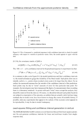
Figure 8.4 Plot of measured vs. predicted responses (with confidence intervals) to check for model
adequacy with respect to variation in predictor values. Here, the model appears to agree with the
data.

(8.134), the covariance matrix of ˆy(θ)is
T −1 T
2 T
cov[ˆy(θ)] = X| θ M cov(θ) X| θ M = σ X| θ M X X| θ M X| (8.143)
θ M
The 100 × (1 − α)% confidence interval for the predicted response in experiment k is then
1/2
[k] [k] T −1 T
ˆ y (θ) = ˆ y (θ M ) ± sT ν,α/2 X| (X X| θ M ) ( X| ) (8.144)
θ M θ M kk
It is common to plot, as in Figure 8.4, the model predictions and their confidence intervals
vs. the model estimates to gauge the reliability of the fitted model. Such plots allow one to
identify outliers, i.e., points whose residual errors seem to be larger than the others. For an
outlier, the measured response lies far outside of the confidence interval of the prediction.
Such points may be due to “extra” amounts of error for that particular data point. For
example, the investigator may have transposed the digits of a measurement when recording
them in a laboratory notebook. As points with such “extra” error corrupt the analysis, they
should be removed from the data set. Of course, we should not discard such points based on
our subjective expectation of the outcome, as outliers that are actually valid, but have large
residuals due to model error, have been known to change the course of scientific history. If
possible, redo any experiments that appear to be outliers. If the excessive error appears to
be reproducible, it may be due to model inadequacy.

Least-squares fitting and confidence interval generation in MATLAB
The MATLAB statistics toolkit contains several functions that perform least-squares param-
eter fits and generate confidence intervals for linear and nonlinear models from single-
response data.