Page 412 - Numerical Methods for Chemical Engineering

Confidence intervals from the approximate posterior density 401

y hat = feval(fun name, theta, X pred);
that returns the vector of predicted responses y hat for input values of the parameters theta
and the predictor values in X pred. theta 0 is an initial guess of the parameter vector.
theta is the least-squares estimate of the parameter vector. residuals contains the residual
errors, and Jac contains the Jacobian of the model functions (i.e. the linearized design
matrix).
ν a ν b
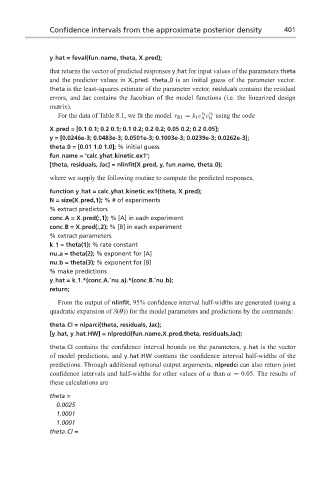
For the data of Table 8.1, we fit the model r R1 = k 1 c c using the code
A B
X pred = [0.1 0.1; 0.2 0.1; 0.1 0.2; 0.2 0.2; 0.05 0.2; 0.2 0.05];
y = [0.0246e-3; 0.0483e-3; 0.0501e-3; 0.1003e-3; 0.0239e-3; 0.0262e-3];
theta 0 = [0.01 1.0 1.0]; % initial guess
fun name = ‘calc yhat kinetic ex1’;
[theta, residuals, Jac] = nlinfit(X pred, y, fun name, theta 0);
where we supply the following routine to compute the predicted responses,
function y hat = calc yhat kinetic ex1(theta, X pred);
N = size(X pred,1); % # of experiments
% extract predictors
conc A=X pred(:,1); % [A] in each experiment
conc B=X pred(:,2); % [B] in each experiment
% extract parameters
k 1 = theta(1); % rate constant
nu a = theta(2); % exponent for [A]
nu b = theta(3); % exponent for [B]
% make predictions
y hat=k 1.*(conc A.ˆnu a).*(conc B.ˆnu b);
return;
From the output of nlinfit, 95% confidence interval half-widths are generated (using a
quadratic expansion of S(θ)) for the model parameters and predictions by the commands:

theta CI = nlparci(theta, residuals, Jac);
[y hat, y hat HW] = nlpredci(fun name,X pred,theta, residuals,Jac);

theta CI contains the confidence interval bounds on the parameters, y hat is the vector
of model predictions, and y hat HW contains the confidence interval half-widths of the
predictions. Through additional optional output arguments, nlpredci can also return joint
confidence intervals and half-widths for other values of α than α = 0.05. The results of
these calculations are

theta =
0.0025
1.0001
1.0001
theta CI =