Page 405 - Numerical Methods for Chemical Engineering

394 8 Bayesian statistics and parameter estimation

2
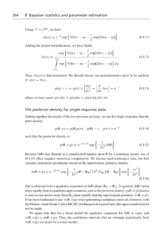
Using s = e 2lns ,wehave
ν
9 :
l(η|s) ∝ s −N exp N(ln s − η) − exp[2(ln s − η)] (8.111)
2
Adding the proper normalization, we have finally
ν
9 :
exp N(ln s − η) − exp[2(ln s − η)]
2
l(η|s) = (8.112)
η max
ν
'
9 :
exp N(ln s − η) − exp[2(ln s − η)] dη
2
η min
Thus, l(η|s) is data-translated. We should choose our noninformative prior to be uniform
in η(σ) = ln σ,

d
dη −1
p(η) ∼ c ⇒ p(σ) ∝ = ln σ = σ (8.113)

dσ dσ
where we have used p(σ)dσ = p(η)dη = p(η) |dη/dσ| dσ.
The posterior density for single-response data

Putting together the results of the two previous sections, we use for single-response data the
prior density

p(θ,σ) = p(θ)p(σ) p(θ) ∼ c p(σ) ∝ σ −1 (8.114)

such that the posterior density is
1
1
−(N+1)
p(θ,σ|y) ∝ σ exp − S(θ) (8.115)
2σ 2
Because S(θ) may depend in a complicated manner upon θ for a nonlinear model, use of
(8.115) often requires numerical computation. We discuss such techniques later, but first
consider analytical calculations based on the approximate posterior density

1 T T νs
1 2 1
−(N+1)
π(θ,σ|y) ∝ σ exp − (θ − θ M ) [X X| θ M ](θ − θ M ) exp −
2σ 2 2σ 2
(8.116)
that is obtained from a quadratic expansion of S(θ) about θ M = θ LS . In general, S(θ) varies
more rapidly than its quadratic approximation, and so the posterior density p(θ,σ|y) decays
to zero as one moves away from θ M more rapidly than the approximate posterior π(θ,σ|y).
It has been traditional to use π(θ,σ|y) when generating confidence intervals; however, with
theMarkovchainMonteCarlo(MCMC)techniquesdiscussedlater,thisapproximationneed
not be made.
We again note that for a linear model the quadratic expansion for S(θ) is exact, and
π(θ,σ|y) = p(θ,σ|y). Thus, the confidence intervals that we compute analytically from
π(θ,σ|y) are exact for a linear model.