Page 419 - Numerical Methods for Chemical Engineering

408 8 Bayesian statistics and parameter estimation

12

1

θ 2

2

−1 − 1 1 2 2
θ 2
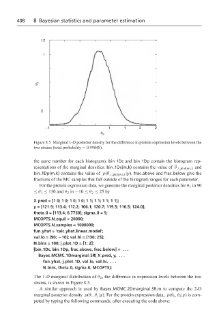
Figure 8.5 Marginal 1-D posterior density for the difference in protein expression levels between the
two strains (total probability = 0.99848).

the same number for each histogram). bin 1Dc and bin 1Dp contain the histogram rep-
resentations of the marginal densities. bin 1Dc(m,k) contains the value of θ j plot(m),k and
bin 1Dp(m,k) contains the value of p(θ j plot(m),k |y). frac above and frac below give the
fractions of the MC samples that fall outside of the histogram ranges for each parameter.
For the protein expression data, we generate the marginal posterior densities for θ 1 in 90
≤ θ 1 ≤ 130 and θ 2 in −10 ≤ θ 2 ≤ 25 by

X pred=[10;10;10;10;11;11;11;11];
y = [121.9; 113.4; 112.2; 106.1; 120.7; 119.5; 116.5; 124.0];
theta 0 = [113.4; 6.7750]; sigma 0=5;
MCOPTS.N equil = 20000;
MCOPTS.N samples = 1000000;
fun yhat = ‘calc yhat linear model’;
val lo = [90; −10]; val hi = [130; 25];
N bins = 100; j plot 1D = [1; 2];
[bin 1Dc, bin 1Dp, frac above, frac below] = . . .
Bayes MCMC 1Dmarginal SR( X pred, y, . . .
fun yhat, j plot 1D, val lo, val hi, . . .
N bins, theta 0, sigma 0, MCOPTS);
The 1-D marginal distribution of θ 2 , the difference in expression levels between the two
strains, is shown in Figure 8.5.
A similar approach is used by Bayes MCMC 2Dmarginal SR.m to compute the 2-D
marginal posterior density p(θ i ,θ j |y). For the protein expression data, p(θ 1 ,θ 2 |y) is com-
puted by typing the following commands, after executing the code above: